GOES-R EXIS Code Example: Using ncagg

Jamie Mothersbaugh, University of Colorado CIRES and NOAA NCEI

This script provides a demonstration of the Python ncagg library, using the GOES-8 XRS data as an example. A month of daily 1-minute average files are aggregated into a single file. The irradiance from the monthly file is then plotted, and the file is examined to check that the aggregation has filled in all missing timestamps.

Code Documentation

GitHub ncagg repository: https://github.com/5tefan/ncagg

ncagg documentation: https://ncagg.readthedocs.io/en/latest/

ncagg is a Python function that aggregates multiple individual NetCDF files into a single combined NetCDF file. The GOES XRS data consists of daily, yearly and mission-length files for each satelite. As shown in this example, ncagg can be used to combine the daily files into single files that span the duration of interest.

Python Initialization

import netCDF4 as nc
import ncflag
# Import libraries to read the NetCDF data files and the data quality flags.

import numpy as np
# Import numpy.

import cftime
import datetime
# Import libraries used to read and plot the data timestamps.

import matplotlib.pyplot as plt
import matplotlib.dates as mdates
import matplotlib.ticker as tck
# Import matplotlib and specific libraries used for formatting the tick marks on the x-axis of the plots.

import requests
import os
from bs4 import BeautifulSoup
import glob
# Import libraries to download the data files.

import ncagg
from ncagg import aggregate
from ncagg.config import Config
# Import NetCDF file aggregation libraries.

# The ncagg library is not a common Python library. It may be necessary to run "pip install ncagg" in the Jupyter Notebook form of this
# script to install ncagg in the Python environment before importing it to the notebook.

# The ncagg library uses pkg_resources, which is part of the setuptools library that is used in this Git repository. pkg_resources has been
# deprecated in setuptools version > 82. The environment.yml file in this repository sets setuptools<82, but there may still be a
# deprecation warning that appears when ncagg is imported to the local Python environment.

/home/runner/micromamba/envs/goesr-spwx-examples/lib/python3.12/site-packages/ncagg/attributes.py:8: UserWarning: pkg_resources is deprecated as an API. See https://setuptools.pypa.io/en/latest/pkg_resources.html. The pkg_resources package is slated for removal as early as 2025-11-30. Refrain from using this package or pin to Setuptools<81.
  import pkg_resources

Example

First, the necessary data files must be downloaded from the GOES 8-15 XRS data website. The code below checks the directory in which this Jupyter Notebook is running; if the necessary files are in this directory, they do not need to be downloaded.

local_directory = './'
xrs_data_website = 'https://www.ncei.noaa.gov/data/goes-space-environment-monitor/access/science/xrs/goes08/xrsf-l2-avg1m_science/2003/05/'
xrs_filename_prefix = 'sci_xrsf-l2-avg1m_g08_d200305'
local_files = sorted(glob.glob(local_directory + xrs_filename_prefix + '*.nc'))
if local_files:
    print('The following data files exist in the local working directory:')
    print(local_files)
else:
    print('Downloading files from the GOES 8-15 XRS data website')
    url = requests.get(xrs_data_website)
    if url.status_code == 200:
        url_files = BeautifulSoup(url.text, 'html.parser')
        for link in url_files.find_all('a'):
            xrs_file = link.get('href')
            if xrs_file and xrs_file.startswith(xrs_filename_prefix) and xrs_file.endswith('.nc'):
                with open(local_directory + xrs_file, "wb") as f:
                    r = requests.get(xrs_data_website + xrs_file)
                    f.write(r.content)
    local_files = sorted(glob.glob(local_directory + xrs_filename_prefix + '*.nc'))
# Check if the May 2003 XRS data files exist in the local working directory. If the files do not exist in the local working directory,
# they will be downloaded to the local working directory from the GOES 8-15 XRS data website.

The following data files exist in the local working directory:
['./sci_xrsf-l2-avg1m_g08_d20030505_v1-0-0.nc', './sci_xrsf-l2-avg1m_g08_d20030506_v1-0-0.nc', './sci_xrsf-l2-avg1m_g08_d20030507_v1-0-0.nc', './sci_xrsf-l2-avg1m_g08_d20030508_v1-0-0.nc', './sci_xrsf-l2-avg1m_g08_d20030509_v1-0-0.nc', './sci_xrsf-l2-avg1m_g08_d20030510_v1-0-0.nc', './sci_xrsf-l2-avg1m_g08_d20030512_v1-0-0.nc', './sci_xrsf-l2-avg1m_g08_d20030513_v1-0-0.nc', './sci_xrsf-l2-avg1m_g08_d20030514_v1-0-0.nc', './sci_xrsf-l2-avg1m_g08_d20030515_v1-0-0.nc', './sci_xrsf-l2-avg1m_g08_d20030516_v1-0-0.nc', './sci_xrsf-l2-avg1m_g08_d20030517_v1-0-0.nc', './sci_xrsf-l2-avg1m_g08_d20030518_v1-0-0.nc', './sci_xrsf-l2-avg1m_g08_d20030519_v1-0-0.nc', './sci_xrsf-l2-avg1m_g08_d20030520_v1-0-0.nc', './sci_xrsf-l2-avg1m_g08_d20030521_v1-0-0.nc', './sci_xrsf-l2-avg1m_g08_d20030522_v1-0-0.nc', './sci_xrsf-l2-avg1m_g08_d20030523_v1-0-0.nc', './sci_xrsf-l2-avg1m_g08_d20030524_v1-0-0.nc', './sci_xrsf-l2-avg1m_g08_d20030525_v1-0-0.nc', './sci_xrsf-l2-avg1m_g08_d20030526_v1-0-0.nc', './sci_xrsf-l2-avg1m_g08_d20030527_v1-0-0.nc', './sci_xrsf-l2-avg1m_g08_d20030528_v1-0-0.nc', './sci_xrsf-l2-avg1m_g08_d20030529_v1-0-0.nc', './sci_xrsf-l2-avg1m_g08_d20030530_v1-0-0.nc']

The aggregation parameters can be set in the code before the files are aggregated. The configuration adjustments below set the header for the aggregated file and specify the timestamp cadence.

The default/expected frequency of data in the ncagg function is 1 Hz (1 timestamp per second). The cadence variable has units of seconds and is the time cadence of the files that are being aggregated. This cadence must be set when aggregating data with a different time cadence than the default. For example, to aggregate 1-minute files, set cadence = 60.0.

first_timestamp = datetime.datetime(2003, 5, 1, 0, 0)
last_timestamp = datetime.datetime(2003, 5, 31, 23, 59)
# Set the first and last timestamps of the aggregated file.
# This example uses the GOES-8 May 2003 data, which does not have data on May 1 or May 31. The start and end timestamps for the aggregated
# file are manually defined, instead of being read from the daily files.

cadence = 60.0
# Set the cadence of the data, in seconds. This value is used as 1/cadence to set the frequency of data in the aggregation.

aggregation_config = Config.from_nc(local_files[0])
aggregation_config.dims["time"].update({"index_by":"time", "min":first_timestamp, "max":last_timestamp})
aggregation_config.dims["time"]["expected_cadence"].update({"time": (1.0 / cadence)})
# Update the aggregation config parameters with the first & last timestamps and time cadence of the dataset.
# This is necessary for filling the data gaps.

# With these two configuration parameter adjustments, ncagg will write a timestamp at the specified cadence at every timestamp between
# the start and end times. There will not be any time gaps in the aggregated file.

Now that the aggregation parameters are defined, the daily files can be aggregated into a single monthly file.

The syntax of the aggregate() call is as follows: aggregate(list_of_files_to_aggregate, name_of_aggregated_file_with_output_path, configuration_parameters)

aggregate(local_files, './sci_xrsf-l2-avg1m_g08_m200305_v1-0-0.nc', aggregation_config)
# Aggregate the data into a single monthly file and write to the local directory.

There are several ways to validate the monthly data. First, read the file back in to Python and print some attributes from the header.

monthly_file = nc.Dataset('./sci_xrsf-l2-avg1m_g08_m200305_v1-0-0.nc')
# Read in the aggregated file and set the 'r+' flag to allow for writing new information & data to the arrays.

print(monthly_file.dimensions)
print(monthly_file.id)
print(monthly_file.date_created)
# Print the selected header attributes to check the size and identifiers of the aggregated file.

{'time': "<class 'netCDF4.Dimension'>" (unlimited): name = 'time', size = 44640}
sci_xrsf-l2-avg1m_g08_d20030505_v1-0-0.nc
2026-07-11T16:16:13.956Z

The date_created attribute shows the file was written now, and the id attribute shows the filename of the aggregation. The dimensions attribute shows the file has 44640 indices. There are 1440 indices each day at a 1-minute cadence, so 1440 * 31 = 44640, the same size as the file.

The first file, and thus the first day with irradiance data, in the aggregation is May 5. As explained above, the configuration parameters defined the start of the aggregation to be 00:00 on May 1. This can be checked in the aggregation.

Next, check the first day of the timestamps array to verify the aggregation contains timestamps without corresponding irradiance data. At a cadence of 1 minute, 1 day is 1440 indices.

timestamps = cftime.num2pydate(monthly_file["time"][:], monthly_file["time"].units)
# Convert timestamps to datetime objects.

print(timestamps[0:1440])
print('')
print('Masked XRS-A irradiance array:')
print(monthly_file["xrsa_flux"][0:1440])

[real_datetime(2003, 5, 1, 0, 0) real_datetime(2003, 5, 1, 0, 1)
 real_datetime(2003, 5, 1, 0, 2) ... real_datetime(2003, 5, 1, 23, 57)
 real_datetime(2003, 5, 1, 23, 58) real_datetime(2003, 5, 1, 23, 59)]

Masked XRS-A irradiance array:
[-- -- -- ... -- -- --]

The first 1440 timestamps of the aggregation are indeed on May 1. The corresponding irradiance values in the XRS-A irradiance array are set to fill values, denoted by “–”, indicating there is no irradiance at these timestamps.

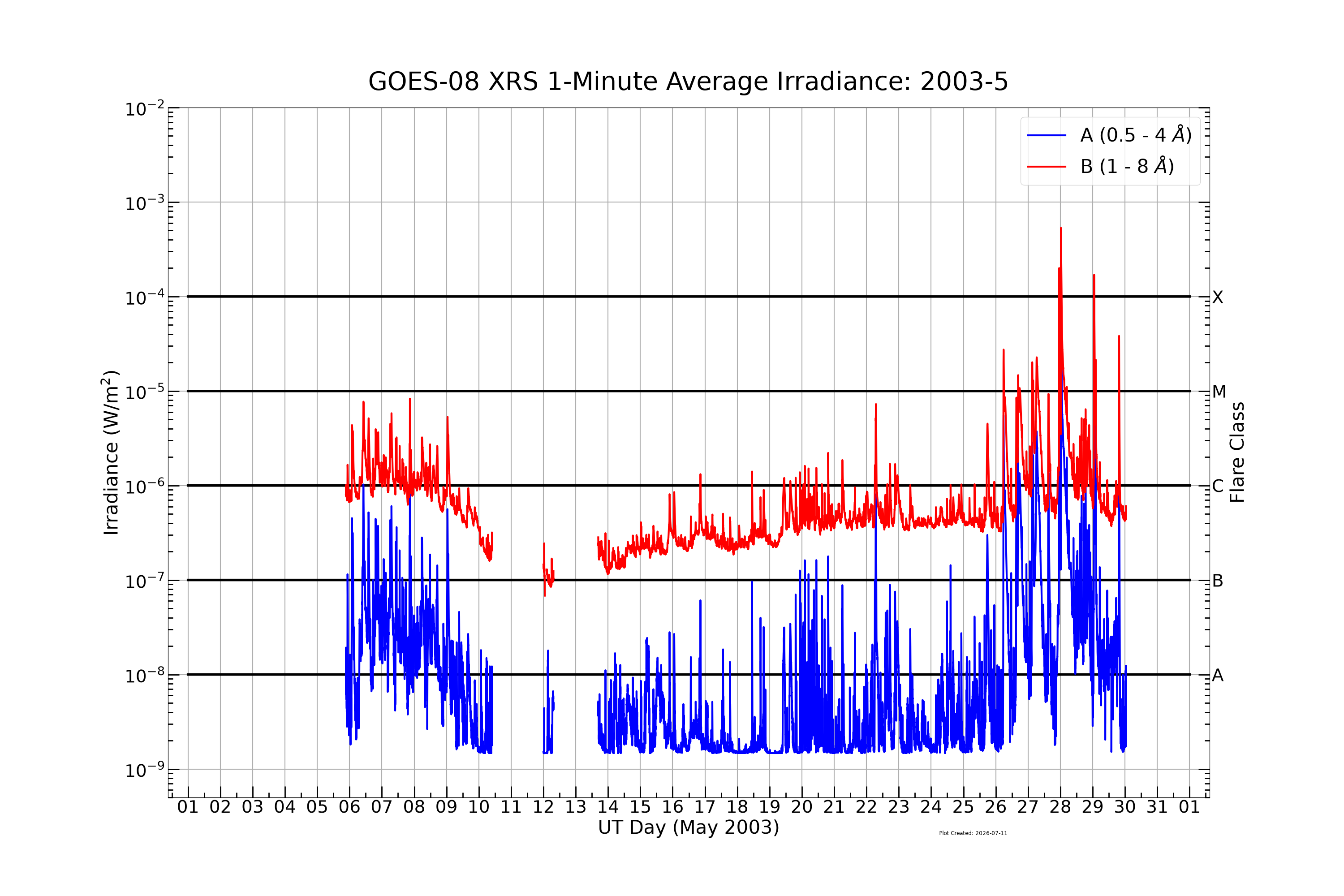
The final check of the aggregation is to plot the XRS-A and XRS-B irradiance. This shows how the aggregated data is organized in the month-long file, and that the aggregation does not contain time gaps.

First, define arrays containing the XRS-A and XRS-B irradiance. These arrays are defined such that, for timestamps at which the irradiances are fill values in the NetCDF file, the values are changed to NaNs, which will not appear on the plot.

xrsa_irrad = np.ma.filled(monthly_file["xrsa_flux"][:], np.nan)
xrsb_irrad = np.ma.filled(monthly_file["xrsb_flux"][:], np.nan)
# Replace irradiance fill & missing values with NaN values in the XRS-A & XRS-B irradiance arrays.

Now plot the XRS-A and XRS-B irradiance and flare class lines.

plt.figure(figsize = (30, 20))
plt.grid(which = 'major', axis = 'both', linewidth = 1.5)
# Major and minor axis grid lines on the plot.

aflare_line = np.repeat(1e-8, len(timestamps), axis = 0)
bflare_line = np.repeat(1e-7, len(timestamps), axis = 0)
cflare_line = np.repeat(1e-6, len(timestamps), axis = 0)
mflare_line = np.repeat(1e-5, len(timestamps), axis = 0)
xflare_line = np.repeat(1e-4, len(timestamps), axis = 0)
plt.plot(timestamps, aflare_line, color = 'black', linewidth = 4, linestyle = 'solid')
plt.plot(timestamps, bflare_line, color = 'black', linewidth = 4, linestyle = 'solid')
plt.plot(timestamps, cflare_line, color = 'black', linewidth = 4, linestyle = 'solid')
plt.plot(timestamps, mflare_line, color = 'black', linewidth = 4, linestyle = 'solid')
plt.plot(timestamps, xflare_line, color = 'black', linewidth = 4, linestyle = 'solid')
plt.plot(timestamps, xrsa_irrad, color = 'blue', linestyle = 'solid', linewidth = 3, label = 'A (0.5 - 4 ' + r'$\AA$' + ')')
plt.plot(timestamps, xrsb_irrad, color = 'red', linestyle = 'solid', linewidth = 3, label = 'B (1 - 8 ' + r'$\AA$' + ')')
# Plot flare class lines behind the irradiance. The flare class lines allow easy identification of the large flares in the GOES-8 May 2003
# data.

plt.yscale('log')
#plt.rc('font', size = 22)
plt.xlabel('UT Day (May 2003)', fontsize = 30)
plt.ylabel('Irradiance (W/m$^2$)', fontsize = 30)
plt.tick_params(axis = 'x', which = 'major', length = 18, width = 2, direction = 'in')
plt.tick_params(axis = 'x', which = 'minor', length = 8, width = 2, direction = 'in')
plt.tick_params(axis = 'y', which = 'major', length = 18, width = 2, direction = 'in')
plt.tick_params(axis = 'y', which = 'minor', length = 8, width = 2, direction = 'in')
plt.gca().xaxis.set_major_formatter(mdates.DateFormatter('%d'))
plt.gca().xaxis.set_major_locator(mdates.DayLocator())
plt.gca().xaxis.set_minor_locator(mdates.HourLocator(12))
plt.xticks(fontsize = 28)
plt.yticks(fontsize = 28)
plt.legend(loc = 'best', fontsize = 30)
plt.margins(0.02, 0.05)
plt.ylim([5e-10, 1e-2])
plt.title(monthly_file.platform + ' XRS 1-Minute Average Irradiance: ' + str(timestamps[0].year) + '-' + str(timestamps[0].month), \
          fontsize = 40, y = 1.02)
plt.text(x = timestamps[round(0.75 * len(timestamps))], y = 2e-10, s = \
         f"Plot Created: {datetime.datetime.now(datetime.UTC).strftime('%Y-%m-%d')}", fontsize = "small")
# Set the axis parameters, labels and plot text.

yflaremag = [1e-9, 1e-8, 1e-7, 1e-6, 1e-5, 1e-4, 1e-3, 1e-2]
yflarelabel = ['', 'A', 'B', 'C', 'M', 'X', '', '']
plt.twinx()
plt.yscale('log')
plt.ylim([5e-10, 1e-2])
plt.yticks(yflaremag, yflarelabel, fontsize = 28)
plt.tick_params(axis = 'y', which = 'major', length = 18, width = 2, direction = 'in')
plt.tick_params(axis = 'y', which = 'minor', length = 8, width = 2, direction = 'in')
plt.ylabel('Flare Class', fontsize = 30)
# Add a righthand y-axis that labels the flare class lines.

Text(2744.416666666667, 0.5, 'Flare Class')

The monthly aggregated file spans the entire month, does not contain data gaps and preserves the irradiance from the daily files.

monthly_file.close()
# Close the NetCDF file.

Additional Example: Changing Header Attributes

The configuration parameters defined above work very well for setting the time cadence and time range in the aggregated file. However, they do not allow for detailed or special case writing in the header attributes. The configuration parameters use the header attributes from the first or last files in the list of files to aggregate. Thus, header attributes like id, input_files_first and input_files_last reference individual file parameters, instead of the entire aggregation.

When writing aggregated files, it is often useful to update certain header attributes so the metadata reflects the actual content of the file. This can be done in Python. Read the aggregated file into Python and set the ‘r+’ flag in the nc.Dataset() function to allow the file to be written from Python.

This example adjusts the orbital_slot and header attributes in the aggregated monthly file.

monthly_file = nc.Dataset('./sci_xrsf-l2-avg1m_g08_m200305_v1-0-0.nc', 'r+')
# Read in the aggregated file.

The orbital_slot and comment header attributes contain the orbital position (“GOES-East”, “GOES-West”, etc.) and the orbital longitude of the satellite on each day of data. These can change if the satellite is moved to a different orbit. When daily files are aggregated into a longer time range, it can be necessary to preserve the orbital information for each day to track changes in the spacecraft across the aggregation time range.

The code below utilizes the daily file list and other parameters of the aggregated data set to change the information in several of the header attributes. These changes are written directly to the aggregated file variable in Python, and can be immediately viewed without saving and re-opening the file.

longitude_list = []
orbital_slot_list = []
for i in np.arange(len(local_files)):
    daily_file = nc.Dataset(local_files[i])
    longitude_list.append(daily_file.comment[0:4])
    orbital_slot_list.append(daily_file.orbital_slot[0:10])
    daily_file.close()
# Make arrays of the orbital slot & longitude values to put in the aggregated file header.

monthly_file.algorithm = 'goesr_exis_ncagg.ipynb'
monthly_file.input_files_first = local_files[0].split('/')[-1]
monthly_file.input_files_last = local_files[-1].split('/')[-1]
monthly_file.input_files_total = len(local_files)
monthly_file.id = 'sci_xrsf-l2-avg1m_g08_m200305_v1-0-0.nc'
monthly_file.time_coverage_start = timestamps[0].strftime("%Y-%m-%d %H:%M") + ' UTC'
monthly_file.time_coverage_end = timestamps[-1].strftime("%Y-%m-%d %H:%M") + ' UTC'
monthly_file.orbital_slot = 'Daily Satellite Position = ' + str(orbital_slot_list)
monthly_file.comment = 'Daily Satellite Longitude (degrees West) = ' + str(longitude_list)
monthly_file.comment_2 = 'Data Source: Daily 1-minute files'
# Adjust header attributes to reflect the daily files used to create the monthly aggregation.
# When the aggregated file is initially made, these fields only show the values from the first file in the file glob.

The changes are written directly to the header and can be immediately viewed in Python.

print(monthly_file.input_files_first)
print(monthly_file.input_files_last)
print(monthly_file.time_coverage_start)
print(monthly_file.time_coverage_end)
print(monthly_file.orbital_slot)
print(monthly_file.comment)
# Print selected header attributes.

sci_xrsf-l2-avg1m_g08_d20030505_v1-0-0.nc
sci_xrsf-l2-avg1m_g08_d20030530_v1-0-0.nc
2003-05-01 00:00 UTC
2003-05-31 23:59 UTC
Daily Satellite Position = ['GOES-East ', 'GOES-East ', 'GOES-East ', 'GOES-East ', 'GOES-East ', 'GOES-East ', 'GOES-East ', 'GOES-East ', 'GOES-East ', 'GOES-East ', 'GOES-East ', 'GOES-East ', 'GOES-East ', 'GOES-East ', 'GOES-East ', 'GOES-East ', 'GOES-East ', 'GOES-East ', 'GOES-East ', 'GOES-East ', 'GOES-East ', 'GOES-East ', 'GOES-East ', 'GOES-East ', 'GOES-East ']
Daily Satellite Longitude (degrees West) = ['76.7', '76.8', '76.9', '76.9', '77.0', '77.1', '89.4', '90.5', '91.5', '92.6', '93.6', '94.7', '95.7', '96.8', '97.9', '98.9', '100.', '101.', '102.', '103.', '104.', '105.', '106.', '107.', '108.']

The orbital_slot attribute now shows the orbital position for each day in the aggregation. The comment attribute shows the orbital longitude for each day in the aggregation. May 2003 is the final month of GOES-8 XRS data. The longitude values clearly change as the satellite moved from the GOES-East position to a non-operational storage orbit. GOES-8 was designated as the GOES-East satellite even as it was moved to the storage orbit.

The input_files_first, input_files_last, input_files_total, time_coverage_start and time_coverage_end attributes now show the correct time ranges and start/stop times of the aggregation.

monthly_file.close()
# Close the NetCDF file. The header changes are now written and saved to the file, and will appear when the file is read in again.