Note
Go to the end to download the full example code.
Opening and Using the XRS Flare Report (CSV)
- Purpose:
Use Python to open and explore the contents of the XRS flare report.
Overview
In this example, we will explain how to use the XRS flare report (flrpt) product, as well as provide examples of how someone might use this data.
- The flare report is an aggregation of the following products:
1997 - current: Space Weather Prediction Center (SWPC) solar event reports
Pre-1997: GOES XRS historical reports
GOES XRS L2 Science Flare Summary (flsum)
GOES XRS L2 Science Flare Location (flloc)
This product was developed to be a singular composite source of solar flare event data. This product will aggregate of GOES-08 - GOES-19 flare events (GOES-01 - GOES-07 to be added at a later date), combined with relevant flare locations from both GOES and SWPC.
NOTE: SWPC’s flare locations are provided to them through the Solar Observing Optical Network (SOON). SWPC occasionally corrects this data manually to better align with active regions or correct errors.
The flare report is available both as a NetCDF file and a CSV file. This example will cover how you can use our CSV Flare Report product, with optional metadata.
Imports
First, we will import the necessary libraries for using this file:
__authors__ = "elucas"

import matplotlib.pyplot as plt
import matplotlib.dates as mdates
import matplotlib.ticker as ticker
import pandas as pd
from datetime import datetime, timedelta
from astropy.coordinates import SkyCoord
import sunpy
import sunpy.map
import astropy.units as u
from sunpy.coordinates import frames
from sunpy.net import Fido, attrs as a
from astropy.io import fits
from IPython.display import display
import json
import requests
import re
import os
Downloading the Flare Report
Relevant data files can be downloaded by running the code below, or downloading manually here. Other data links and information about EXIS data can be found here.
This section will download the mission-length flare report from the web.
download_dir = "./"
base_url = "https://data.ngdc.noaa.gov/platforms/solar-space-observing-satellites/goes/multi/l2/data/xrsf-l2-flrpt_science/csv/"

# get HTML text
response = requests.get(base_url)
html_content = response.text

# this looks for the specific prefix of the mission-length aggregate CSV
pattern = r'sci_xrsf-l2-flrpt_geo_s\d+_e\d+_v[\d\-]+\.csv'
match = re.search(pattern, html_content)
if match:
    file_to_download = match.group(0)
    flrpt_local_path = os.path.join(download_dir, file_to_download)

    print(f"File found: {file_to_download}. Downloading...")
    try:
        file_data = requests.get(base_url + file_to_download).content
        with open(flrpt_local_path, "wb") as f:
            f.write(file_data)
        print(f"File download successful.")
    except:
        print(f"File download failed.")
else:
    print("No matching file found on online.")
File found: sci_xrsf-l2-flrpt_geo_s19950103_e20260709_v1-0-1.csv. Downloading...
File download successful.
This section will download the optional metadata JSON file.
download_dir = "./"
base_url = "https://data.ngdc.noaa.gov/platforms/solar-space-observing-satellites/goes/multi/l2/data/xrsf-l2-flrpt_science/csv/"

# get HTML text
response = requests.get(base_url)
html_content = response.text

# this looks for the associated metadata JSON file
pattern = r'sci_xrsf-l2-flrpt_geo_metadata.json'
match = re.search(pattern, html_content)
if match:
    file_to_download = match.group(0)
    json_local_path = os.path.join(download_dir, file_to_download)

    print(f"File found: {file_to_download}. Downloading...")
    try:
        file_data = requests.get(base_url + file_to_download).content
        with open(json_local_path, "wb") as f:
            f.write(file_data)
        print(f"File download successful.")
    except:
        print(f"File download failed.")
else:
    print("No matching file found on online.")
File found: sci_xrsf-l2-flrpt_geo_metadata.json. Downloading...
File download successful.
Reading in the Flare Report
pd.set_option("display.max_columns", None)

# Read the .csv flare report into a pandas dataframe, and convert time to datetime (can also do this with start and end).
df = pd.read_csv(flrpt_local_path)
df['time'] = pd.to_datetime(df['time'])
display(df)
/home/runner/work/goesr-spwx-examples/goesr-spwx-examples/examples/exis/flrpt_example_csv.py:129: DtypeWarning: Columns (0: flare_loc_xrs_source) have mixed types. Specify dtype option on import or set low_memory=False.
  df = pd.read_csv(flrpt_local_path)
                     time           start_time             end_time  \
0     1995-01-03 00:14:00  1995-01-03 00:04:00  1995-01-03 00:19:00
1     1995-01-03 00:49:00  1995-01-03 00:43:00  1995-01-03 00:54:00
2     1995-01-03 01:03:00  1995-01-03 00:58:00  1995-01-03 01:07:00
3     1995-01-03 01:21:00  1995-01-03 01:13:00  1995-01-03 01:30:00
4     1995-01-03 02:05:00  1995-01-03 02:00:00  1995-01-03 02:13:00
...                   ...                  ...                  ...
81007 2026-07-09 05:25:00  2026-07-09 05:17:00  2026-07-09 05:30:00
81008 2026-07-09 07:13:00  2026-07-09 06:51:00  2026-07-09 07:35:00
81009 2026-07-09 13:38:00  2026-07-09 13:35:00                  NaN
81010 2026-07-09 13:49:00  2026-07-09 13:46:00  2026-07-09 13:51:00
81011 2026-07-09 15:47:00  2026-07-09 15:33:00  2026-07-09 15:58:00

           flare_id    xrsb_irrad flare_class xrsb_irrad_source  \
0      199501030004  8.629000e-07        B8.6            GOES-8
1      199501030043  2.429000e-07        B2.4            GOES-8
2      199501030058  2.571000e-07        B2.5            GOES-8
3      199501030113  3.343000e-07        B3.3            GOES-8
4      199501030200  2.514000e-07        B2.5            GOES-8
...             ...           ...         ...               ...
81007  202607090517  6.675000e-07        B6.6           GOES-18
81008  202607090651  2.706000e-06        C2.7           GOES-18
81009  202607091335  7.229000e-07        B7.2           GOES-18
81010  202607091346  7.352000e-07        B7.3           GOES-18
81011  202607091533  7.105000e-07        B7.1           GOES-18

       background_irrad  integrated_irrad_peak  integrated_irrad_end  \
0          1.786000e-07               0.000342              0.000429
1          1.496000e-07               0.000123              0.000158
2          1.820000e-07               0.000119              0.000145
3          2.009000e-07               0.000195              0.000313
4          1.521000e-07               0.000111              0.000183
...                 ...                    ...                   ...
81007      5.951000e-07               0.000460              0.000572
81008      6.243000e-07               0.002776              0.005276
81009      3.622000e-07               0.000231                   NaN
81010      5.353000e-07               0.000269              0.000304
81011      4.140000e-07               0.000635              0.000962

       flare_loc_swpc_hgs_lon  flare_loc_swpc_hgs_lat flare_loc_swpc_source  \
0                         NaN                     NaN                   NaN
1                         NaN                     NaN                   NaN
2                         NaN                     NaN                   NaN
3                         NaN                     NaN                   NaN
4                         NaN                     NaN                   NaN
...                       ...                     ...                   ...
81007                     NaN                     NaN                   NaN
81008                    29.0                   -14.0                   LEA
81009                     NaN                     NaN                   NaN
81010                     NaN                     NaN                   NaN
81011                    37.0                   -10.0                   HOL

       flare_loc_xrs_hgs_lon  flare_loc_xrs_hgs_lat  flare_loc_xrs_hpc_x  \
0                        NaN                    NaN                  NaN
1                        NaN                    NaN                  NaN
2                        NaN                    NaN                  NaN
3                        NaN                    NaN                  NaN
4                        NaN                    NaN                  NaN
...                      ...                    ...                  ...
81007                    NaN                    NaN                  NaN
81008              21.209984             -20.874733             320.1925
81009                    NaN                    NaN                  NaN
81010                    NaN                    NaN                  NaN
81011                    NaN                    NaN                  NaN

       flare_loc_xrs_hpc_y flare_loc_xrs_source  sequential_flare_num  \
0                      NaN                  NaN                     1
1                      NaN                  NaN                     1
2                      NaN                  NaN                     1
3                      NaN                  NaN                     1
4                      NaN                  NaN                     1
...                    ...                  ...                   ...
81007                  NaN                  NaN                     2
81008           -390.45648          GOES-18_XRS                     1
81009                  NaN                  NaN                     1
81010                  NaN                  NaN                     2
81011                  NaN                  NaN                     1

       event_id_swpc  peak_saturated  active_region
0                NaN               0            NaN
1                NaN               0            NaN
2                NaN               0            NaN
3                NaN               0            NaN
4                NaN               0            NaN
...              ...             ...            ...
81007         6960.0               0         4485.0
81008         6990.0               0         4485.0
81009            NaN               0            NaN
81010         7010.0               0         4482.0
81011         7040.0               0         4485.0

[81012 rows x 22 columns]
# Read the metadata into a dictionary.
with open(json_local_path, 'r') as f:
    metadata = json.load(f)
display(json.dumps(metadata, indent=4))
{
    "global_attributes": {
        "Conventions": "ACDD-1.3, Spase v2.2.6",
        "title": "L2 XRS flare report",
        "summary": "The flare report combines information from both the GOES XRS flare summary files and the SWPC solar event reports. This report provides, for each flare event, the start, peak, and end times, as well as other information such as flare class, irradiances, and flare location.",
        "keywords": "NumericalData.MeasurementType.Irradiance",
        "keywords_vocabulary": "SPASE: Space Physics Archive Search and Extract Data Model version 2.2.6, GCMD: NASA Global Change Master Directory (GCMD) Earth Science Keywords version 8.5",
        "naming_authority": "gov.nesdis.noaa",
        "history": "See algorithm information.",
        "source": "GOES XRS L2 flsum science files, SWPC solar event reports",
        "processing_level": "Level 2",
        "processing_level_description": "Derived products",
        "license": "These data may be redistributed and used without restriction. ",
        "creator_name": "NOAA NCEI STP Solar Irradiance Team",
        "creator_type": "group",
        "creator_institution": "DOC/NOAA/NESDIS/NCEI/COGS/GSDB/STP",
        "creator_email": "goesr.exis@noaa.gov",
        "creator_url": "https://www.ncei.noaa.gov/",
        "institution": "DOC/NOAA/NESDIS",
        "publisher_name": "National Centers for Environmental Information",
        "publisher_type": "institution",
        "publisher_institution": "DOC/NOAA/NESDIS/NCEI",
        "publisher_email": "ncei.info@noaa.gov",
        "publisher_url": "https://www.ncei.noaa.gov/",
        "instrument": "GOES-1 through -19; Solar Observing Optical Network (SOON) ",
        "program": "Geostationary Operational Environmental Satellite, R-Series (GOES-R)",
        "project": "Geostationary Operational Environmental Satellite R-Series (GOES-R) Core Ground Segment, Satellite Product Analysis and Distribution System (SPADES)",
        "time_coverage_resolution": "PT1M",
        "algorithm_parameters": "None",
        "date_created": "2026-07-11 09:02:05.057374",
        "time_coverage_start": "19950103",
        "time_coverage_end": "20260709",
        "flrpt_algorithm_version": "1-0-1"
    },
    "variable_attributes": {
        "time": {
            "long_name": "Record start time for flare peak. Neglects leap seconds since 1970-01-01. ",
            "comments": "Time [UTC] = 1 Jan 1970 00:00:00 [UTC] + time[secs] + n[secs]. To ignore leap seconds, set n = 0. To include leap seconds, set n = number of leap seconds since 1 Jan 1970."
        },
        "start_time": {
            "long_name": "Flare event start time"
        },
        "end_time": {
            "long_name": "Flare event end time",
            "comments": "Time when flare irradiance has declined by 1/2 relative to background."
        },
        "flare_id": {
            "long_name": "SWPC flare identifier",
            "comments": "Unique identifier based on flare event start with format YYYYMMDDHHMM.  Same as in flsum product.",
            "units": "1",
            "valid_min": 0
        },
        "xrsb_irrad": {
            "long_name": "1-minute averaged irradiance for XRS-B",
            "units": "W/m2",
            "valid_min": 9.999999960041972e-12,
            "valid_max": 0.10000000149011612
        },
        "flare_class": {
            "long_name": "Flare class",
            "comments": "Recorded at flare peak."
        },
        "xrsb_irrad_source": {
            "long_name": "Satellite used to measure flare irradiance",
            "units": "1",
            "valid_min": 1,
            "valid_max": 19,
            "flag_values": [
                1,
                2,
                3,
                4,
                5,
                6,
                7,
                8,
                9,
                10,
                11,
                12,
                13,
                14,
                15,
                16,
                17,
                18,
                19
            ],
            "flag_meanings": "GOES-1 GOES-2 GOES-3 GOES-4 GOES-5 GOES-6 GOES-7 GOES-8 GOES-9 GOES-10 GOES-11 GOES-12 GOES-13 GOES-14 GOES-15 GOES-16 GOES-17 GOES-18 GOES-19"
        },
        "background_irrad": {
            "long_name": "Background irradiance",
            "comments": "Recorded at flare start.",
            "units": "W/m2",
            "valid_min": 9.999999717180685e-10,
            "valid_max": 0.10000000149011612
        },
        "integrated_irrad_peak": {
            "long_name": "Integrated irradiance between flare start and peak",
            "units": "J/m2",
            "valid_min": 9.999999717180685e-10
        },
        "integrated_irrad_end": {
            "long_name": "Integrated irradiance between flare start and end",
            "comments": "Integrated irradiance between flare start and end, where flare end is when flare irradiance has declined by 1/2 relative to background.",
            "units": "J/m2",
            "valid_min": 9.999999717180685e-10
        },
        "flare_loc_swpc_hgs": {
            "long_name": "Flare location in heliographic Stonyhurst coordinates (lon, lat) from ground-based observatories or GOES-12 SXI. Data obtained from SWPC solar event reports.",
            "comments": "Values for on-disk flares only.",
            "units": "degrees, degrees",
            "valid_min": -180.0,
            "valid_max": 180.0
        },
        "flare_loc_swpc_source": {
            "long_name": "Source of flare_loc_swpc_hgs",
            "comments": "Ground stations are Culgoora, Australia (CUL) and Solar Observing Optical Network (SOON) stations: Holloman AFB, USA (HOL); RAAF Learmonth, Australia (LEA); Ramey AFB, Puerto Rico, USA (RAM); San Vito dei Normanni Air Station, Italy (SVI); and combined (COM) multiple ground stations. Satellite flare locations are from GOES-12 Solar X-Ray Imager (SXI) or SDO Atmospheric Imaging Assembly (AIA) 193nm channel.",
            "units": "1",
            "valid_min": 0,
            "valid_max": 7,
            "flag_values": [
                0,
                1,
                2,
                3,
                4,
                5,
                6,
                7
            ],
            "flag_meanings": "COM CUL HOL LEA RAM SVI SXI AIA_193"
        },
        "flare_loc_xrs_hgs": {
            "long_name": "Flare location in heliographic Stonyhurst coordinates (lon, lat) provided by satellite",
            "comments": "Values for on-disk flares only.",
            "units": "degrees, degrees",
            "valid_min": -180.0,
            "valid_max": 180.0
        },
        "flare_loc_xrs_hpc": {
            "long_name": "Flare location in helioprojective Cartesian coordinates (x, y) provided by satellite",
            "units": "arcsec, arcsec"
        },
        "flare_loc_xrs_source": {
            "long_name": "Source of flare_loc_xrs_hgs and flare_loc_xrs_hpc",
            "comments": "GOES Satellite X-Ray Sensor (XRS).",
            "units": "1",
            "valid_min": 0,
            "valid_max": 3,
            "flag_values": [
                0,
                1,
                2,
                3
            ],
            "flag_meanings": "GOES-16_XRS GOES-17_XRS GOES-18_XRS GOES-19_XRS"
        },
        "sequential_flare_num": {
            "long_name": "Number in flare sequence",
            "comments": "Flare number for a multiple flare sequence. 0=no flare, 1=first flare, 2=second flare, etc. Incremented at flare start. For previous flare, if peak was <90 minutes earlier and had no flare end, then flare_num>1.",
            "units": "1",
            "valid_min": 1,
            "valid_max": 10
        },
        "event_id_swpc": {
            "long_name": "Flare event ID 'bin' number assigned by SWPC",
            "units": "1",
            "valid_min": 0,
            "valid_max": 9999
        },
        "peak_saturated": {
            "long_name": "Flare peak saturation flag",
            "comments": "Saturation only occurred on GOES-1 through GOES-12.",
            "units": "1",
            "valid_min": 0,
            "valid_max": 1,
            "flag_values": [
                0,
                1
            ],
            "flag_meanings": "unsaturated saturated"
        },
        "active_region": {
            "long_name": "Active region number",
            "units": "1",
            "valid_min": 1,
            "valid_max": 9999
        }
    }
}
Using the data
Here are a few examples of how you might use this data.
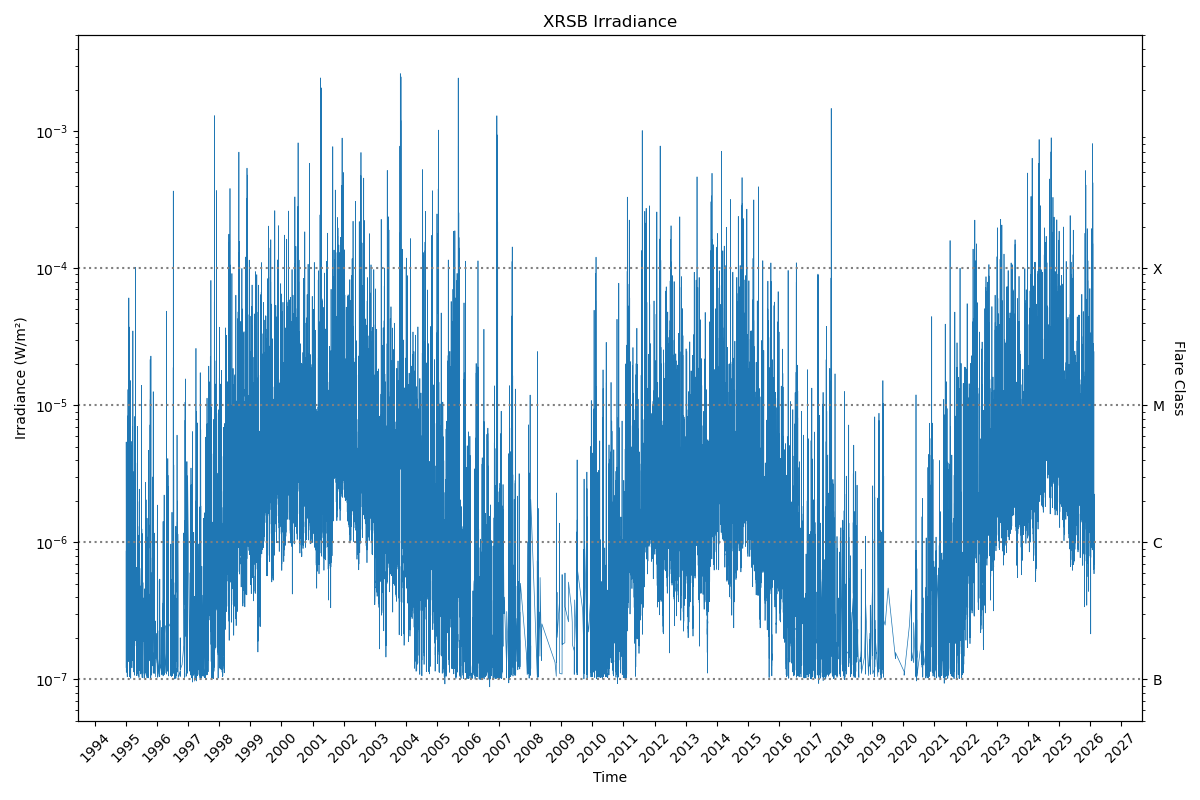
Plot XRS-B Irradiance
# Plot the data
xrsb_irrad = df['xrsb_irrad']
max_times = pd.to_datetime(df['time'])

fig, ax1 = plt.subplots(figsize=(12, 8))

# Plot irradiance data
ax1.plot(max_times, xrsb_irrad, linewidth=0.5)

# Set parameters for the left y-axis
ax1.set_yscale('log')
ax1.set_ylabel('Irradiance (W/m²)')
ax1.set_xlabel('Time')
ax1.tick_params(axis='x', rotation=45)


# Establish class thresholds
thresholds = {
    'B': 10**-7,
    'C': 10**-6,
    'M': 10**-5,
    'X': 10**-4
}

# Add horizontal lines at the class thresholds
for threshold in thresholds.values():
    ax1.axhline(y=threshold, color='gray', linestyle='dotted')
ax1.set_ylim(min(thresholds.values()) / 2, max(thresholds.values()) * 50)

# Create flare class axis
ax2 = ax1.twinx()
ax2.set_yscale('log')
ax2.set_ylim(ax1.get_ylim())
ax2.set_ylabel('Flare Class', rotation=270, labelpad=15)
ax2.set_yticks(list(thresholds.values()))
ax2.set_yticklabels(list(thresholds.keys()))
ax2.xaxis.set_major_locator(mdates.YearLocator())

plt.title('XRSB Irradiance')
plt.tight_layout()
plt.show()
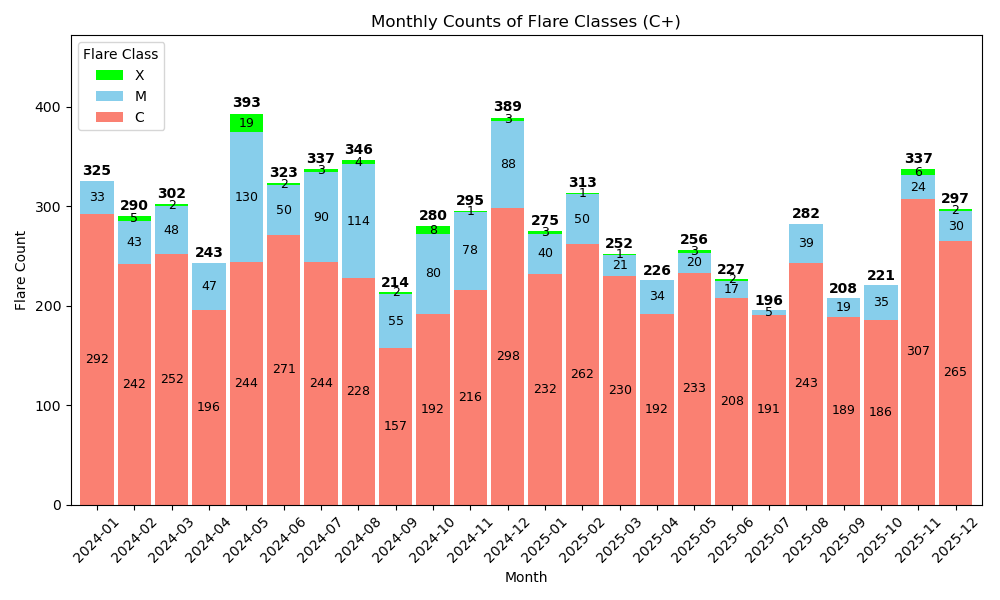
Count Flares in Each Flare Class Between 2024-2025
# Grab flare class letter
df['flare_type'] = df['flare_class'].str[0]

# Group by month and flare type
monthly_counts = df.groupby([pd.Grouper(key='time', freq='ME'), 'flare_type']).size().unstack(fill_value=0)
monthly_counts = monthly_counts.reindex(columns=['C', 'M', 'X'], fill_value=0)

# Limit flare dates
start_date = '2024-01-01'
end_date = '2025-12-31'
monthly_counts = monthly_counts.loc[start_date:end_date]
monthly_counts.index = monthly_counts.index.strftime('%Y-%m')

# Plot stacked bar chart of flare classes
ax = monthly_counts.plot(kind='bar',
                         stacked=True,
                         color=['salmon', 'skyblue', 'lime'],
                         figsize=(10, 6),
                         width=0.9)

plt.xlabel('Month')
plt.ylabel('Flare Count')
plt.title('Monthly Counts of Flare Classes (C+)')
plt.xticks(rotation=45)

# Flip legend so X is on top
handles, labels = ax.get_legend_handles_labels()
ax.legend(list(reversed(handles)), list(reversed(labels)), title='Flare Class', loc='upper left')

# Add annotations for flare class counts
for c in ax.containers:
    labels = [int(v.get_height()) if v.get_height() > 0 else '' for v in c]
    ax.bar_label(c, labels=labels, label_type='center', fontsize=9)

# Add annotations for total flare count (offset by 1% of height to avoid annotation conflicts)
totals = monthly_counts.sum(axis=1)
for i, total in enumerate(totals):
    ax.text(i, 1.01*total, str(total), ha='center', va='bottom', fontsize=10, weight='bold')

# Adjust limits to fit top labels
plt.ylim(0, totals.max() * 1.2)
plt.tight_layout()
plt.show()
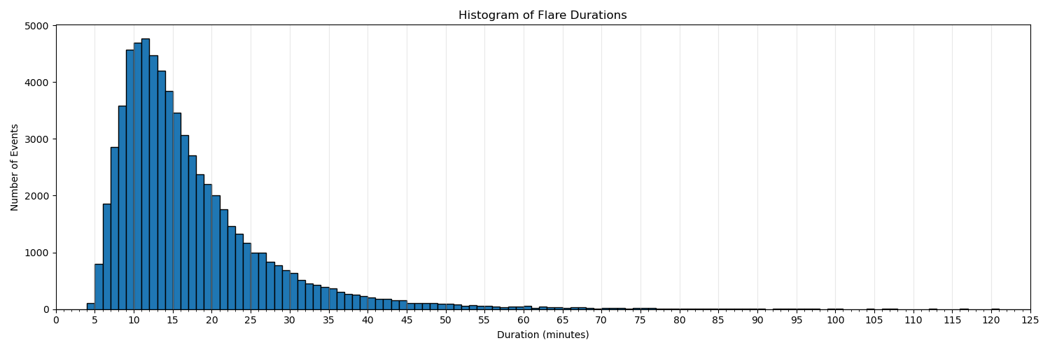
Make a Histogram of Flare Durations
# Plot histogram of end - start times, binned every minute
fig, ax = plt.subplots(figsize=(15, 5))
flare_lengths = (pd.to_datetime(df['end_time']) - pd.to_datetime(df['start_time'])).dt.total_seconds() / 60
bins = range(0, int(flare_lengths.max()) + 5, 1)
plt.hist(flare_lengths, bins=bins, edgecolor='black')

# Add vertical lines every 5 minutes
ax.grid(which='major', axis='x', color='lightgray', linestyle='-', alpha=0.5)

# Set plot parameters
ax.xaxis.set_major_locator(ticker.MultipleLocator(5))
ax.xaxis.set_minor_locator(ticker.MultipleLocator(1))
plt.xlim(0, 125)
plt.xlabel('Duration (minutes)')
plt.ylabel('Number of Events')
plt.title('Histogram of Flare Durations')
plt.tight_layout()
plt.show()
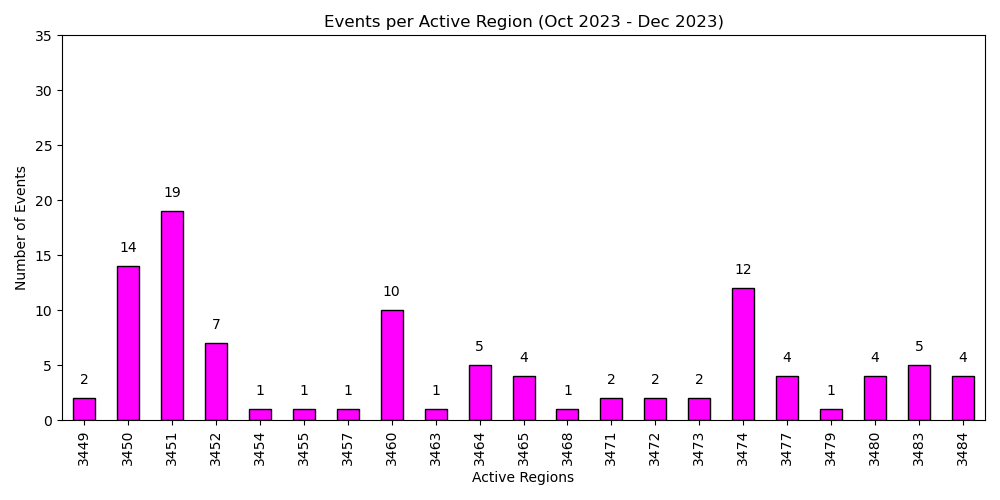
Count occurrences of each active region from Oct 2023 - Dec 2023
fig, ax = plt.subplots(figsize=(10, 5))

# Grab event counts between for 10/1/2023 - 12/1/2023
event_counts = df['active_region'][(pd.to_datetime(df['start_time']) >= datetime(2023, 10, 1, 0, 0)) &
                                   (pd.to_datetime(df['end_time']) <= datetime(2023, 12, 1, 0, 0))].value_counts()
event_counts = event_counts.sort_index(ascending=True)

# Plot bar chart
ax = event_counts.plot(kind='bar', color='magenta', edgecolor='black')
plt.xlabel('Active Regions')
plt.ylabel('Number of Events')
plt.title('Events per Active Region (Oct 2023 - Dec 2023)')
ax.set_xticklabels(event_counts.index.astype(int), rotation=90)
ax.set_ylim(0, 35)

# Add count to each bar
for i, count in enumerate(event_counts):
    plt.text(i, count + 1, str(count), ha='center', va='bottom', fontsize=10, color='black')

plt.tight_layout()
plt.show()
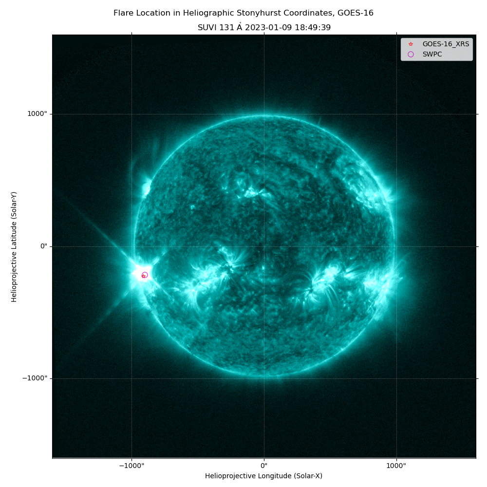
Plot Heliographic Stonyhurst Flare Locations
Retrieve the corresponding SUVI SunPy Map
# Get flare event for requested time
flloc_time = datetime(2023, 1, 9, 18, 50)
event = df[pd.to_datetime(df['time']) == flloc_time]
goes = int(event['flare_loc_xrs_source'].values[0].split('-')[1].split('_')[0])
flloc_swpc = [float(event['flare_loc_swpc_hgs_lon'].values[0]), float(event['flare_loc_swpc_hgs_lat'].values[0])]
flloc_goes = [float(event['flare_loc_xrs_hgs_lon'].values[0]), float(event['flare_loc_xrs_hgs_lat'].values[0])]

# Pull down closest SUVI SunPy Map for 2023-01-09 18:50, +- 2 minutes
def create_suvi_sunpymap(date, goes=16, wavelength=131, rng=2):
    ds0 = (date - timedelta(minutes=rng)).strftime("%Y/%m/%d %H:%M:%S")
    ds1 = (date + timedelta(minutes=rng)).strftime("%Y/%m/%d %H:%M:%S")
    q = Fido.search(a.Time(ds0, ds1), a.Instrument.suvi, a.Wavelength(wavelength*u.angstrom))
    tmp_files = Fido.fetch(q)

    # Select only files for level 2 composites from G16
    for tmp_file in tmp_files:
        if (f'g{goes}' in tmp_file) and ('l2' in tmp_file):
            data, header = fits.getdata(tmp_file, ext=1), fits.getheader(tmp_file, ext=1)
            suvi_map = sunpy.map.Map(data, header)
            return suvi_map, data, header
    print('No SUVI map available')
    return None


# Access SUVI SunPy map for requested time
suvi_map, suvi_data, suvi_header = create_suvi_sunpymap(flloc_time, goes=goes)
/home/runner/micromamba/envs/goesr-spwx-examples/lib/python3.12/site-packages/sunpy/net/vso/vso.py:206: SunpyUserWarning: VSO-D400 Bad Request - Invalid wavelength, wavetype of filter specification
  warn_user(resp["error"])

Files Downloaded:   0%|          | 0/16 [00:00<?, ?file/s]


OR_SUVI-L1b-Fe131_G16_s20230091849487_e20230091849487_c20230091850098.fits.gz:   0%|          | 0.00/1.27M [00:00<?, ?B/s]

OR_SUVI-L1b-Fe131_G16_s20230091849397_e20230091849407_c20230091850004.fits.gz:   0%|          | 0.00/1.53M [00:00<?, ?B/s]


OR_SUVI-L1b-Fe131_G16_s20230091849487_e20230091849487_c20230091850128.fits.gz:   0%|          | 0.00/1.27M [00:00<?, ?B/s]


OR_SUVI-L1b-Fe131_G16_s20230091849397_e20230091849407_c20230091850030.fits.gz:   0%|          | 0.00/1.53M [00:00<?, ?B/s]


OR_SUVI-L1b-Fe131_G16_s20230091849587_e20230091849587_c20230091850191.fits.gz:   0%|          | 0.00/1.34M [00:00<?, ?B/s]


OR_SUVI-L1b-Fe131_G16_s20230091849487_e20230091849487_c20230091850128.fits.gz:   0%|          | 1.02k/1.27M [00:00<02:58, 7.12kB/s]


OR_SUVI-L1b-Fe131_G16_s20230091849487_e20230091849487_c20230091850098.fits.gz:   0%|          | 1.02k/1.27M [00:00<03:14, 6.54kB/s]


OR_SUVI-L1b-Fe131_G16_s20230091849587_e20230091849587_c20230091850191.fits.gz:   0%|          | 1.02k/1.34M [00:00<03:07, 7.11kB/s]

OR_SUVI-L1b-Fe131_G16_s20230091849397_e20230091849407_c20230091850004.fits.gz:   0%|          | 1.02k/1.53M [00:00<03:53, 6.55kB/s]


OR_SUVI-L1b-Fe131_G16_s20230091849397_e20230091849407_c20230091850030.fits.gz:   0%|          | 1.02k/1.53M [00:00<03:51, 6.61kB/s]


OR_SUVI-L1b-Fe131_G16_s20230091849487_e20230091849487_c20230091850098.fits.gz:  20%|██        | 257k/1.27M [00:00<00:00, 1.22MB/s]


OR_SUVI-L1b-Fe131_G16_s20230091849487_e20230091849487_c20230091850128.fits.gz:  14%|█▍        | 184k/1.27M [00:00<00:01, 878kB/s]


OR_SUVI-L1b-Fe131_G16_s20230091849397_e20230091849407_c20230091850030.fits.gz:  14%|█▍        | 216k/1.53M [00:00<00:01, 1.03MB/s]

OR_SUVI-L1b-Fe131_G16_s20230091849397_e20230091849407_c20230091850004.fits.gz:  14%|█▍        | 217k/1.53M [00:00<00:01, 959kB/s]


OR_SUVI-L1b-Fe131_G16_s20230091849587_e20230091849587_c20230091850191.fits.gz:  14%|█▍        | 193k/1.34M [00:00<00:01, 833kB/s]


OR_SUVI-L1b-Fe131_G16_s20230091849487_e20230091849487_c20230091850098.fits.gz:  78%|███████▊  | 988k/1.27M [00:00<00:00, 3.68MB/s]


OR_SUVI-L1b-Fe131_G16_s20230091849487_e20230091849487_c20230091850128.fits.gz:  77%|███████▋  | 979k/1.27M [00:00<00:00, 3.71MB/s]


OR_SUVI-L1b-Fe131_G16_s20230091849397_e20230091849407_c20230091850030.fits.gz:  61%|██████▏   | 940k/1.53M [00:00<00:00, 3.48MB/s]

OR_SUVI-L1b-Fe131_G16_s20230091849397_e20230091849407_c20230091850004.fits.gz:  66%|██████▌   | 1.01M/1.53M [00:00<00:00, 3.54MB/s]


Files Downloaded:   6%|▋         | 1/16 [00:00<00:08,  1.80file/s]


OR_SUVI-L1b-Fe131_G16_s20230091849587_e20230091849587_c20230091850191.fits.gz:  73%|███████▎  | 977k/1.34M [00:00<00:00, 3.39MB/s]


dr_suvi-l2-ci131_g16_s20230109T184800Z_e20230109T185200Z_v1-0-1.fits:   0%|          | 0.00/1.85M [00:00<?, ?B/s]


OR_SUVI-L1b-Fe131_G16_s20230091849587_e20230091849587_c20230091850225.fits.gz:   0%|          | 0.00/1.34M [00:00<?, ?B/s]


dr_suvi-l2-ci131_g16_s20230109T185200Z_e20230109T185600Z_v1-0-1.fits:   0%|          | 0.00/1.84M [00:00<?, ?B/s]

OR_SUVI-L1b-Fe131_G18_s20230091849283_e20230091849293_c20230091849470.fits.gz:   0%|          | 0.00/1.57M [00:00<?, ?B/s]


OR_SUVI-L1b-Fe131_G18_s20230091849283_e20230091849293_c20230091849491.fits.gz:   0%|          | 0.00/1.57M [00:00<?, ?B/s]


dr_suvi-l2-ci131_g16_s20230109T184800Z_e20230109T185200Z_v1-0-1.fits:   0%|          | 1.02k/1.85M [00:00<04:42, 6.52kB/s]


OR_SUVI-L1b-Fe131_G16_s20230091849587_e20230091849587_c20230091850225.fits.gz:   0%|          | 2.00/1.34M [00:00<30:58:27, 12.0B/s]


dr_suvi-l2-ci131_g16_s20230109T185200Z_e20230109T185600Z_v1-0-1.fits:   0%|          | 1.02k/1.84M [00:00<04:40, 6.56kB/s]

OR_SUVI-L1b-Fe131_G18_s20230091849283_e20230091849293_c20230091849470.fits.gz:   0%|          | 1.02k/1.57M [00:00<03:43, 6.99kB/s]


OR_SUVI-L1b-Fe131_G18_s20230091849283_e20230091849293_c20230091849491.fits.gz:   0%|          | 1.02k/1.57M [00:00<04:00, 6.52kB/s]


dr_suvi-l2-ci131_g16_s20230109T184800Z_e20230109T185200Z_v1-0-1.fits:  12%|█▏        | 224k/1.85M [00:00<00:01, 1.07MB/s]


OR_SUVI-L1b-Fe131_G16_s20230091849587_e20230091849587_c20230091850225.fits.gz:  11%|█         | 145k/1.34M [00:00<00:01, 658kB/s]


dr_suvi-l2-ci131_g16_s20230109T185200Z_e20230109T185600Z_v1-0-1.fits:   9%|▉         | 168k/1.84M [00:00<00:02, 803kB/s]

OR_SUVI-L1b-Fe131_G18_s20230091849283_e20230091849293_c20230091849470.fits.gz:  12%|█▏        | 192k/1.57M [00:00<00:01, 900kB/s]


OR_SUVI-L1b-Fe131_G18_s20230091849283_e20230091849293_c20230091849491.fits.gz:  15%|█▍        | 232k/1.57M [00:00<00:01, 1.10MB/s]


dr_suvi-l2-ci131_g16_s20230109T184800Z_e20230109T185200Z_v1-0-1.fits:  54%|█████▍    | 1.01M/1.85M [00:00<00:00, 3.79MB/s]


dr_suvi-l2-ci131_g16_s20230109T185200Z_e20230109T185600Z_v1-0-1.fits:  48%|████▊     | 879k/1.84M [00:00<00:00, 3.35MB/s]


OR_SUVI-L1b-Fe131_G16_s20230091849587_e20230091849587_c20230091850225.fits.gz:  73%|███████▎  | 981k/1.34M [00:00<00:00, 3.50MB/s]


Files Downloaded:  38%|███▊      | 6/16 [00:01<00:01,  6.04file/s]

OR_SUVI-L1b-Fe131_G18_s20230091849283_e20230091849293_c20230091849470.fits.gz:  64%|██████▍   | 1.01M/1.57M [00:00<00:00, 3.77MB/s]


OR_SUVI-L1b-Fe131_G18_s20230091849283_e20230091849293_c20230091849491.fits.gz:  67%|██████▋   | 1.05M/1.57M [00:00<00:00, 3.96MB/s]


dr_suvi-l2-ci131_g16_s20230109T184800Z_e20230109T185200Z_v1-0-1.fits:  98%|█████████▊| 1.81M/1.85M [00:00<00:00, 5.32MB/s]


Files Downloaded:  62%|██████▎   | 10/16 [00:01<00:00, 10.44file/s]


OR_SUVI-L1b-Fe131_G18_s20230091849373_e20230091849373_c20230091849569.fits.gz:   0%|          | 0.00/1.16M [00:00<?, ?B/s]


OR_SUVI-L1b-Fe131_G18_s20230091849373_e20230091849373_c20230091849591.fits.gz:   0%|          | 0.00/1.16M [00:00<?, ?B/s]


OR_SUVI-L1b-Fe131_G18_s20230091849473_e20230091849473_c20230091850066.fits.gz:   0%|          | 0.00/1.36M [00:00<?, ?B/s]

OR_SUVI-L1b-Fe131_G18_s20230091849473_e20230091849473_c20230091850086.fits.gz:   0%|          | 0.00/1.35M [00:00<?, ?B/s]


dr_suvi-l2-ci131_g18_s20230109T184800Z_e20230109T185200Z_v1-0-1.fits:   0%|          | 0.00/1.81M [00:00<?, ?B/s]


OR_SUVI-L1b-Fe131_G18_s20230091849373_e20230091849373_c20230091849569.fits.gz:   0%|          | 1.02k/1.16M [00:00<03:09, 6.09kB/s]


OR_SUVI-L1b-Fe131_G18_s20230091849373_e20230091849373_c20230091849591.fits.gz:   0%|          | 1.02k/1.16M [00:00<02:57, 6.53kB/s]

OR_SUVI-L1b-Fe131_G18_s20230091849473_e20230091849473_c20230091850086.fits.gz:   0%|          | 2.00/1.35M [00:00<29:22:34, 12.8B/s]


OR_SUVI-L1b-Fe131_G18_s20230091849473_e20230091849473_c20230091850066.fits.gz:   0%|          | 1.02k/1.36M [00:00<03:44, 6.04kB/s]


dr_suvi-l2-ci131_g18_s20230109T184800Z_e20230109T185200Z_v1-0-1.fits:   0%|          | 1.02k/1.81M [00:00<04:35, 6.57kB/s]


OR_SUVI-L1b-Fe131_G18_s20230091849373_e20230091849373_c20230091849569.fits.gz:  12%|█▏        | 144k/1.16M [00:00<00:01, 649kB/s]


OR_SUVI-L1b-Fe131_G18_s20230091849373_e20230091849373_c20230091849591.fits.gz:  20%|█▉        | 230k/1.16M [00:00<00:00, 1.09MB/s]


OR_SUVI-L1b-Fe131_G18_s20230091849473_e20230091849473_c20230091850066.fits.gz:   9%|▉         | 128k/1.36M [00:00<00:02, 582kB/s]


dr_suvi-l2-ci131_g18_s20230109T184800Z_e20230109T185200Z_v1-0-1.fits:  10%|█         | 182k/1.81M [00:00<00:01, 869kB/s]

OR_SUVI-L1b-Fe131_G18_s20230091849473_e20230091849473_c20230091850086.fits.gz:  11%|█         | 144k/1.35M [00:00<00:01, 637kB/s]


OR_SUVI-L1b-Fe131_G18_s20230091849373_e20230091849373_c20230091849569.fits.gz:  74%|███████▍  | 859k/1.16M [00:00<00:00, 3.20MB/s]


OR_SUVI-L1b-Fe131_G18_s20230091849373_e20230091849373_c20230091849591.fits.gz:  85%|████████▌ | 989k/1.16M [00:00<00:00, 3.56MB/s]


OR_SUVI-L1b-Fe131_G18_s20230091849473_e20230091849473_c20230091850066.fits.gz:  65%|██████▌   | 881k/1.36M [00:00<00:00, 3.24MB/s]


dr_suvi-l2-ci131_g18_s20230109T184800Z_e20230109T185200Z_v1-0-1.fits:  50%|████▉     | 905k/1.81M [00:00<00:00, 3.45MB/s]

OR_SUVI-L1b-Fe131_G18_s20230091849473_e20230091849473_c20230091850086.fits.gz:  53%|█████▎    | 721k/1.35M [00:00<00:00, 2.56MB/s]


Files Downloaded:  81%|████████▏ | 13/16 [00:01<00:00,  8.05file/s]


dr_suvi-l2-ci131_g18_s20230109T185200Z_e20230109T185600Z_v1-0-1.fits:   0%|          | 0.00/1.43M [00:00<?, ?B/s]


dr_suvi-l2-ci131_g18_s20230109T184800Z_e20230109T185200Z_v1-0-1.fits:  98%|█████████▊| 1.77M/1.81M [00:00<00:00, 5.15MB/s]


dr_suvi-l2-ci131_g18_s20230109T185200Z_e20230109T185600Z_v1-0-1.fits:   0%|          | 1.02k/1.43M [00:00<03:21, 7.07kB/s]


dr_suvi-l2-ci131_g18_s20230109T185200Z_e20230109T185600Z_v1-0-1.fits:  15%|█▍        | 209k/1.43M [00:00<00:01, 1.00MB/s]


dr_suvi-l2-ci131_g18_s20230109T185200Z_e20230109T185600Z_v1-0-1.fits:  75%|███████▍  | 1.06M/1.43M [00:00<00:00, 4.04MB/s]


Files Downloaded: 100%|██████████| 16/16 [00:02<00:00,  7.30file/s]
Files Downloaded: 100%|██████████| 16/16 [00:02<00:00,  7.16file/s]
Plot GOES-16 and SWPC Heliographic Stonyhurst Coordinates
# Plot the SUVI SunPy composite image
fig_hg = plt.figure(figsize=(10, 10))
fig_hg.tight_layout(h_pad=-50)
fig_hg.suptitle(f'Flare Location in Heliographic Stonyhurst Coordinates, GOES-{goes}')
ax_hg = fig_hg.add_subplot(projection=suvi_map)
suvi_map.plot(axes=ax_hg, clip_interval=(0.1, 99.9) * u.percent)
num_points = 100

# Note: Ignore INFO message about 'Missing metadata for solar radius: assuming the standard radius of the photosphere.'

#~~~~~~ GOES-16 Flare Location ~~~~~~#
# Convert flare location into SkyCoord object in coordinate frame
flloc_hgs_sc = SkyCoord(flloc_goes[0] * u.degree, flloc_goes[1] * u.degree, obstime=flloc_time, observer=suvi_map.observer_coordinate,
                        frame=frames.HeliographicStonyhurst)

# Transform SkyCoord object to the SUVI SunPy map's coordinate frame
flloc_hgs_sc = flloc_hgs_sc.transform_to(suvi_map.coordinate_frame)

# Plot flare
ax_hg.plot_coord(flloc_hgs_sc, color='r', marker='*', fillstyle='none', linestyle='none', markersize=6, alpha=0.7, label=event['flare_loc_xrs_source'].values[0])


#~~~~~~ SWPC Flare Location ~~~~~~#
# Convert flare location into SkyCoord object in coordinate frame
flloc_hgs_sc_s = SkyCoord(flloc_swpc[0] * u.degree, flloc_swpc[1] * u.degree, obstime=flloc_time, observer=suvi_map.observer_coordinate,
                        frame=frames.HeliographicStonyhurst)

# Transform SkyCoord object to the SUVI SunPy map's coordinate frame
flloc_hgs_sc_s = flloc_hgs_sc_s.transform_to(suvi_map.coordinate_frame)

# Plot flare
ax_hg.plot_coord(flloc_hgs_sc_s, color='m', marker='o', fillstyle='none', linestyle='none', markersize=8, alpha=0.7, label='SWPC')

# Add legend for features
plt.legend()
plt.tight_layout()
plt.show()
INFO: Missing metadata for solar radius: assuming the standard radius of the photosphere. [sunpy.map.mapbase]
2026-07-11 16:16:34 - sunpy - INFO: Missing metadata for solar radius: assuming the standard radius of the photosphere.
INFO: Missing metadata for solar radius: assuming the standard radius of the photosphere. [sunpy.map.mapbase]
2026-07-11 16:16:35 - sunpy - INFO: Missing metadata for solar radius: assuming the standard radius of the photosphere.
Total running time of the script: (0 minutes 20.450 seconds)