Using Quality Flags

This script demonstrates how to use the ncflag library to work with flags embedded in xrs data.

In this example, we will be examining one day of high resolution 1-second data from the GOES-16 XRS. XRS is measuring x-ray irradiance from the sun. We’ll summarize the flags, remove particle spikes, and zoom in on an eclipse period where the Earth comes between the instrument and the sun and blocks the x-ray signal.

Useful links:

• The ncflag library (https://github.com/5tefan/ncflag, pip install ncflag or conda install ncflag)

• The cf conventions (http://cfconventions.org/cf-conventions/cf-conventions.html#flags) which explain how quality flags are encoded with metadata.

As a general note, we recommend using the metadata in the files. For example, we discourage you from creating your own time conversion functions, instead you should use the cftime library (https://github.com/Unidata/cftime) which is also available from the netCDF library as nc.num2date(arr, units). Use the units from the units attribute of the time variable, as demonstrated below. We also discourage you from handling flags by hard coding bit masks. There is no guarantee that these bit positions will always remain the same. New flag_meanings may be added in the future. Your code should use the flag_meanings, flag_masks, and flag_values attributes associated with the flag variables… the ncflag library does this for you, as demonstrated below.

import matplotlib.pyplot as plt
from ncflag import FlagWrap
import netCDF4 as nc
import numpy as np

import cftime

# For fetching data...
import os
import requests

• The data can be downloaded and browsed here.

• Other data links and information about EXIS data can be found here

filename = "sci_xrsf-l2-flx1s_g16_d20200929_v2-2-0.nc"

# Download `filename` if it does not exist locally
if not os.path.exists(filename):
    with open(filename, "wb") as f:
        url_path = "https://data.ngdc.noaa.gov/platforms/solar-space-observing-satellites/goes/goes16/l2/data/xrsf-l2-flx1s_science/2020/09/"
        r = requests.get(url_path + filename)
        f.write(r.content)

Open and read some data from the netcdf file.

with nc.Dataset(filename) as nc_in:
    times = cftime.num2pydate(nc_in.variables["time"][:], nc_in.variables["time"].units)
    xrsb_flags = FlagWrap.init_from_netcdf(nc_in.variables["xrsb_flags"])
    xrsb_flux = np.ma.filled(nc_in.variables["xrsb_flux"][:], fill_value=np.nan)

Let’s inspect what flag_meanings are available, and how many points are flagged for each of these flag meanings

for flag_meaning in xrsb_flags.flag_meanings:
    flags = xrsb_flags.get_flag(flag_meaning)
    num_set = np.count_nonzero(flags)
    print(f"{flag_meaning:<20}: {num_set}")

good_data           : 79165
eclipse             : 4843
particle_spike      : 87
calibration         : 0
off_point           : 2305
temperature_error   : 0
data_quality_error  : 6
pointing_error      : 5895
invalid_mode        : 6
missing_data        : 1
L0_error            : 0

A common task with flags is to get an overview of what flags are signaling at what points in time. It’s convenient to plot this with matplotlib, along with the data.

plt.subplot(2, 1, 1)
plt.semilogy(times, xrsb_flux, linestyle="None", marker=".")
plt.ylabel("xrsb_flux [W/m2]")
plt.subplot(2, 1, 2)
for flag_meaning in xrsb_flags.flag_meanings:
    flags = xrsb_flags.get_flag(flag_meaning)
    if np.any(flags):
        flag_times = times[flags]
        flag_values = [flag_meaning for _ in range(len(flag_times))]
        plt.plot(flag_times, flag_values, ls="None", marker="o")
# Make sure there's room for the long flag_meaning names.
plt.gcf().autofmt_xdate()
plt.xlabel("time UT")
plt.subplots_adjust(left=0.3, right=0.98)
plt.suptitle("xrsb_flux and xrsb_flags")
plt.show()

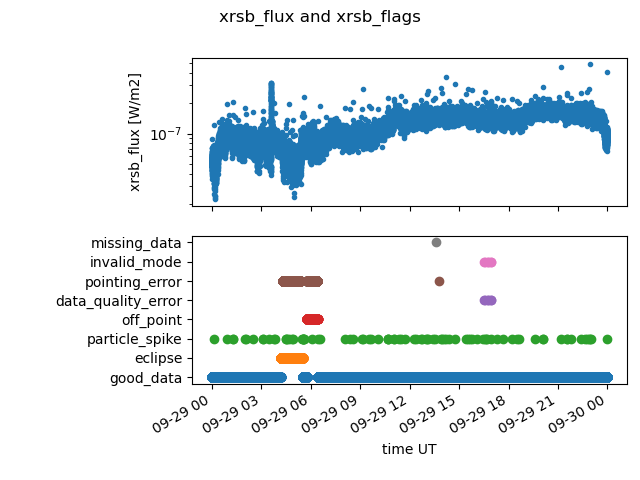
There are a lot of flags on this particular day. (That’s why we picked it for this example!) From the previous plot, some interesting features are visible:

1. There are particle spikes throughout the day.

2. There’s an eclipse early in the day, which is associated with some pointing flags.

3. The instrument appears to have temporarily entered an invalid mode about 3/4 the way through the day.

# Let's pick some portion near the middle of the day and zoom in on some particle spikes.
# We'll plot spikes and non spikes in different colors to see which points are flagged as spikes...

particle_spike = xrsb_flags.get_flag("particle_spike")
plt.semilogy(times[~particle_spike], xrsb_flux[~particle_spike],
             linestyle="None", marker=".", label="not particle_spike")
plt.semilogy(times[particle_spike], xrsb_flux[particle_spike],
             linestyle="None", marker=".", label="particle_spike")

# zoom in on some arbitrary period near the middle of the day...
plt.xlim(times[[30_000, 40_000]])

plt.legend()
plt.suptitle("XRS with particle_spike flagged points highlighted")
plt.xlabel("time UT")
plt.ylabel("irradiance [W/m2]")
plt.show()

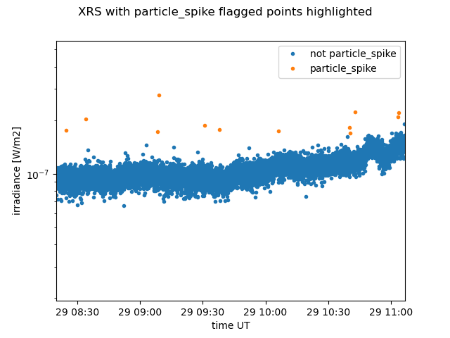
We’re generally not interested in spikes, so let’s replace any point that is flagged as a particle_spike with np.nan so that they are not included in further analysis and don’t show up on plots.

xrsb_flux[particle_spike] = np.nan

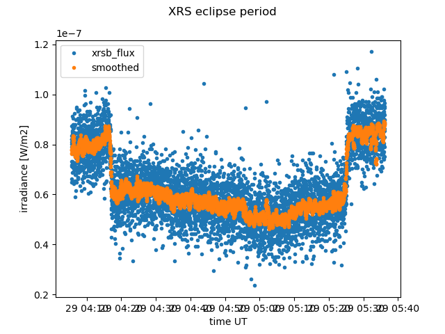
As we saw above, there are are some eclipse flags set. Let’s check out the irradiance observations to verify. The Earth came between the instrument and the sun, so we shouldn’t see as much signal. The remaining signal will be thermal noise and electron contamination.

The eclipse is contiguous, so we’ll just take the start and end, +/- 300 points to include an extra 5 minutes of the irradiance time series on each side, so that we can clearly see the transition into eclipse.

def running_mean(x, n):
    """
    Compute running mean of x with window size of n, handles nan values.

    https://stackoverflow.com/a/27681394

    :param x: 1D array of values
    :param n: window size
    :return: running mean with shape (len(x) - N)
    """
    cumsum = np.nancumsum(np.insert(x, 0, 0))
    return (cumsum[n:] - cumsum[:-n]) / float(n)

eclipse = xrsb_flags.get_flag("eclipse")
eclipse_start_index, eclipse_end_index = np.where(eclipse)[0][[0, -1]]
eclipse_slice = slice(eclipse_start_index - 300, eclipse_end_index + 300)

eclipse_times = times[eclipse_slice]
eclipse_xrsb = xrsb_flux[eclipse_slice]
plt.plot(eclipse_times, eclipse_xrsb,
         linestyle="none", marker=".", label="xrsb_flux")

smoothing_window = 15
eclipse_xrsb_smoothed = running_mean(eclipse_xrsb, smoothing_window)
plt.plot(
    eclipse_times[smoothing_window // 2:-(smoothing_window - 2) // 2],
    eclipse_xrsb_smoothed,
    linestyle="none", marker=".", label="smoothed")

plt.suptitle("XRS eclipse period")
plt.legend()
plt.xlabel("time UT")
plt.ylabel("irradiance [W/m2]")
plt.show()

Eclipses are interesting, but they are not measurements of solar x-ray irradiance. Most users of xrs data will _not_ be interested in eclipsed data. In fact, eclipses and other flagged conditions will distort statistic.

If you’re looking for genuine x-ray irradiance, you should only look at points flagged as good_data. (Even better would be to look at the xrsf-l2-avg1m (1-minute average) product, which attempts to correct for electron contamination!)

# Mean of all data, before taking good_data only.
orig_xrsb_mean = np.nanmean(xrsb_flux)

# set any points that are NOT good_data to nan
good_data = xrsb_flags.get_flag("good_data")
xrsb_flux[~good_data] = np.nan

# Mean of good_data only.
xrsb_mean = np.nanmean(xrsb_flux)

print(f"Mean (all except spikes)             : {orig_xrsb_mean:0.2e} [W/m2]")
print(f"Mean (only good_data)                : {xrsb_mean:0.2e} [W/m2]")
print(f"Difference (good - all except spikes): {xrsb_mean - orig_xrsb_mean:0.2e} [W/m2]")

Mean (all except spikes)             : 1.20e-07 [W/m2]
Mean (only good_data)                : 1.24e-07 [W/m2]
Difference (good - all except spikes): 4.71e-09 [W/m2]