Read and Plot MAG Data With Quality Flags

Download, read and plot 1-Minute Average (avg1m) GOES-R Series Magnetometer (MAG) data and quality flags (DQFs)

Note: this example requires the ncflag python library (pip install ncflag or conda install ncflag). This library reads netCDF data quality flag variables which follow the climate and forecast quality flag conventions.

Import modules

import numpy as np
import matplotlib.pyplot as plt
import cftime
import netCDF4 as nc
from ncflag import FlagWrap
import os, sys, requests

• MAG data (averaged to 1 minute cadence) can be found at the url shown below

• Data links and information can be found here

dataurl = 'https://data.ngdc.noaa.gov/platforms/solar-space-observing-satellites/goes/goes16/l2/data/magn-l2-avg1m'
subdir = '/2021/11/'
filename = "dn_magn-l2-avg1m_g16_d20211115_v2-0-2.nc"

# Download `filename` if it does not exist locally
if not os.path.exists(filename):
    with open(filename, "wb") as f:
        url_path = dataurl+subdir+filename
        print(url_path)
        r = requests.get(url_path)
        f.write(r.content)

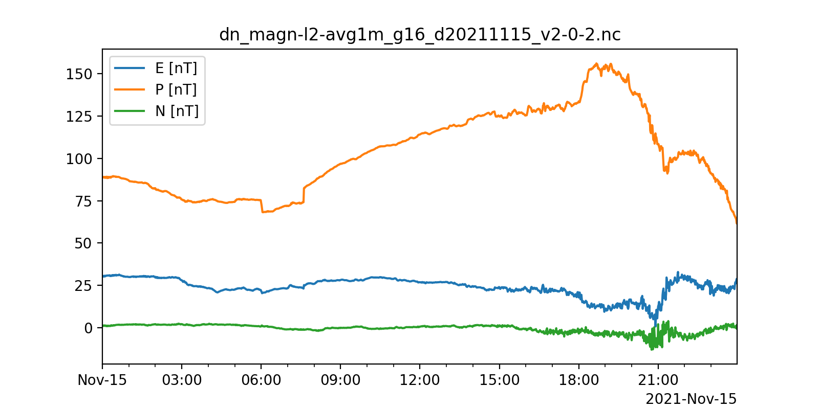
The following demonstrates reading and plotting magnetic field measurements.

def format_time_axis(ax):
    """Helper function; formats x-axis of plot with more readable times"""
    import matplotlib.dates as mdates
    locator = mdates.HourLocator(interval=3)
    ax.xaxis.set_major_locator(locator)
    ax.xaxis.set_minor_locator(mdates.HourLocator())
    ax.xaxis.set_major_formatter(mdates.ConciseDateFormatter(locator))

def read_nctime(ncfn,time_ncvar='time'):
    """Helper function; reads timestamps from a CF-compliant netCDF file
    and converts them to Python datetimes using cftime
    """
    with nc.Dataset(ncfn) as ncf:
        dts = cftime.num2pydate(ncf.variables[time_ncvar][:],
                                ncf.variables[time_ncvar].units)
    return dts

def mag_plot(ax,ncfn):
    """Plot magnetic field in EPN coordinate frame"""
    dts = read_nctime(ncfn)
    with nc.Dataset(filename) as ncf:
        B_epn = ncf['b_epn'][:]
    for cmpntcol,cmpnt in enumerate(['E','P','N']):
        ax.plot(dts,B_epn[:,cmpntcol],label=f'{cmpnt} [nT]')
        ax.legend()
        ax.set_title(filename)
        format_time_axis(ax)
    ax.set_xlim(dts[0],dts[-1])

f,ax = plt.subplots(1,1,figsize=(8,4),dpi=200)
mag_plot(ax,filename)
plt.show()

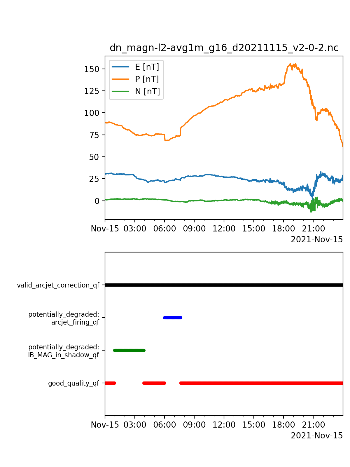
Quality information is available as specific quality flags (following the CF quality flag standard). Note that flags which indicate possibly bad data begin with ‘potentially_degraded_due_to’ and flags which indicate bad data begin with ‘degraded_due_to’. The following demonstrates one way to visualize data quality using quality flags

def read_cfflagvar(ncfn,flag_ncvar):
    """Read the values and required attributes for a
    CF-compliant data quality flag variable using ncflag"""
    with nc.Dataset(ncfn) as ncf:
        intflags = ncf.variables[flag_ncvar][:]
        fmeanings = ncf.variables[flag_ncvar].flag_meanings
        fvalues = ncf.variables[flag_ncvar].flag_values
        fmasks = ncf.variables[flag_ncvar].flag_masks
    return FlagWrap(intflags,fmeanings,fvalues,flag_masks=fmasks)

def flag_plot(ax,ncfn,ncvar,colors=['r', 'g', 'b','k']):
    """Plot CF-compliant data flags
    encoded in netCDF variable
    """
    from itertools import cycle
    #Read data
    t = read_nctime(ncfn)
    fw = read_cfflagvar(ncfn,ncvar)

    #Allocate loop-related variables
    nshown,shown_flag_meanings,shown_flag_labels = 0,[],[]
    nhidden,hidden_flag_meanings = 0,[]
    colorcycle = cycle(colors)

    #Loop over all possible flags
    for flag_key in fw.flag_meanings:
        #Returns a boolean array with True at all times
        #for which the flag is set
        flag_is_set = fw.get_flag(flag_key)
        if np.any(flag_is_set):
            nshown+=1
            shown_flag_meanings.append(flag_key)
            #Reformat long flag names
            if 'due_to' in flag_key:
                flag_label = ':\n'.join(flag_key.split('_due_to_'))
            else:
                flag_label = flag_key
            shown_flag_labels.append(flag_label)

            y = np.full((len(t),),np.nan)
            #plot points at y=nshown, so that they will
            #line up with the label for this flag on the y-axis
            y[flag_is_set] = nshown
            #Plot the data which has this flag set
            ax.plot(t,y,marker='.',linestyle='none',color=next(colorcycle))
        else:
            nhidden+=1
            hidden_flag_meanings.append(flag_key)

    #Format plot
    ax.set_ylim([0,nshown+1])
    ax.set_yticks(np.arange(1,nshown+1),shown_flag_labels,fontsize=8)
    ax.set_xlim(t[0],t[-1])
    format_time_axis(ax)

f,axs = plt.subplots(2,1,figsize=(6,8),dpi=200)
mag_plot(axs[0],filename)
flag_plot(axs[1],filename,'DQF')
#Ensure there is space for long data quality flag names
f.subplots_adjust(left=0.3, right=0.98)
plt.show()