Note
Go to the end to download the full example code.
Plot SUVI L2 Bright Regions
- Purpose:
Use Python to plot SUVI L2 bright region (brght) product in various coordinate systems.
Overview
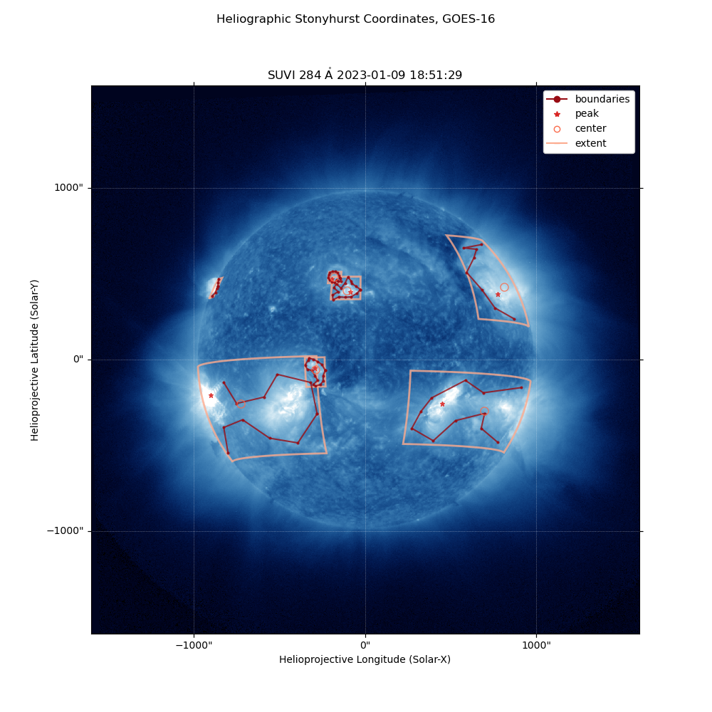
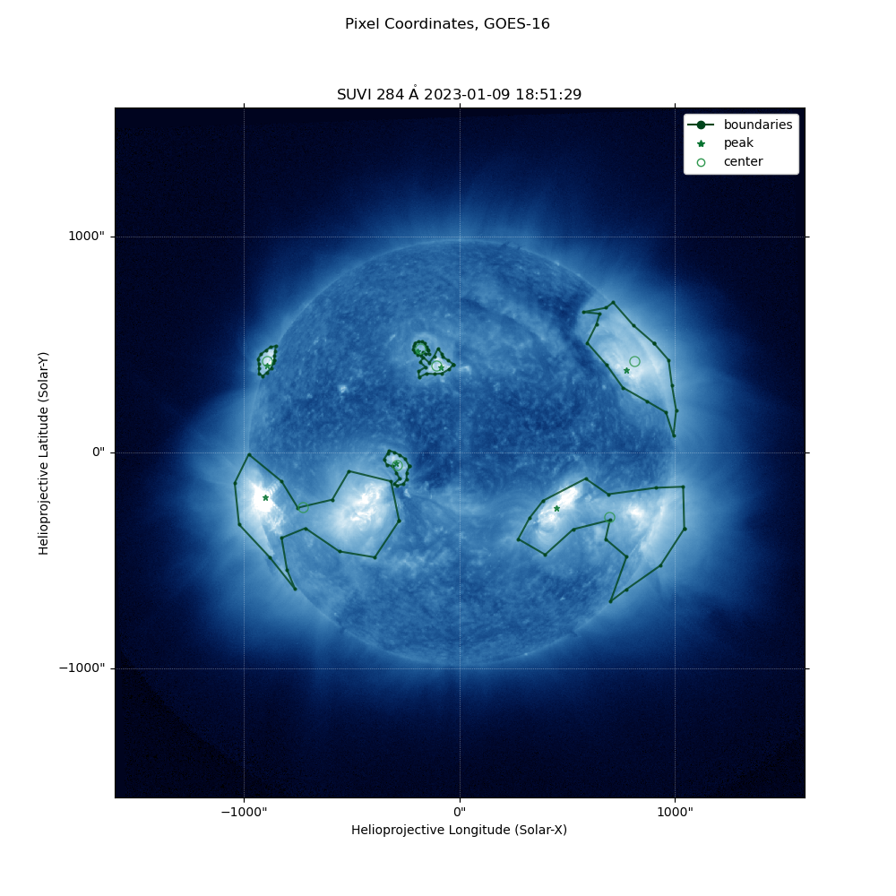
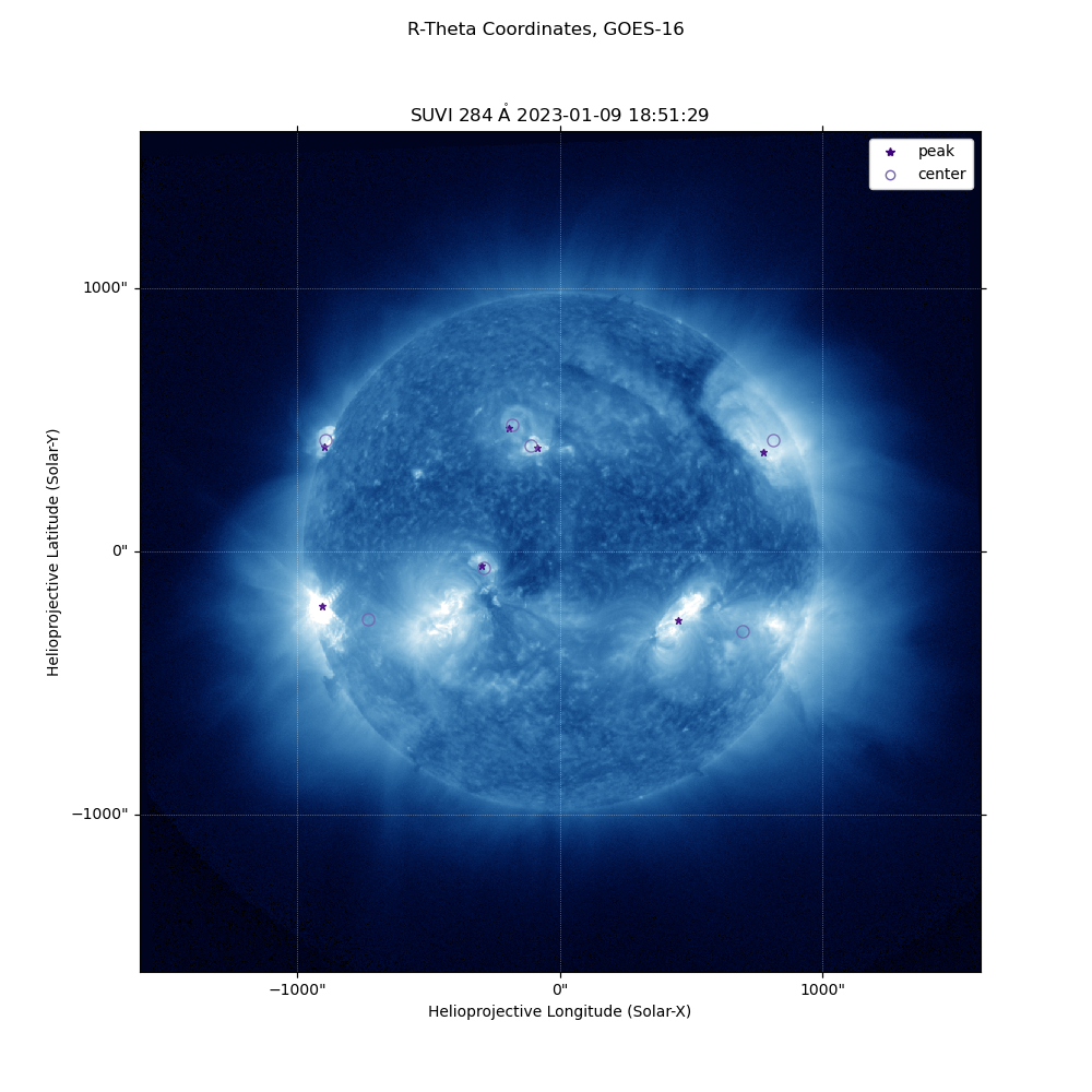
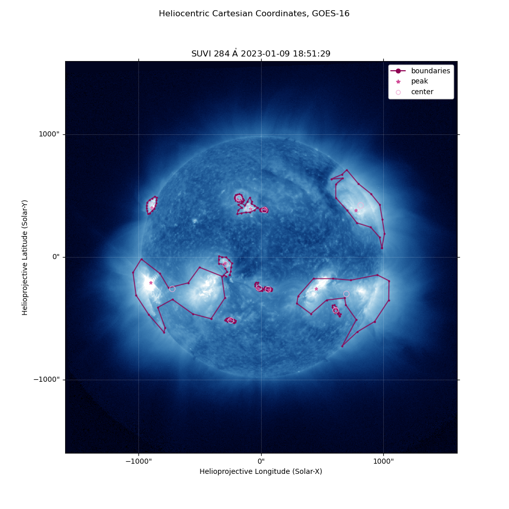
In this example, we will be plotting the bright region boundaries (bnd_loc), center location (center_loc), peak location (peak_loc), and bright region extent (brght_extent) for the bright region report (brght) product. Bright region boundaries outline the bright region, which are akin to coronal active regions. Center location is determined by center-of-mass calculations, whereas peak location is determined by the region with the highest irradiance. The bright region extent is defined by the min/max lat/lon of all vertices of the bright region boundary polygon.
Notes for this product: The extent is only available in the Heliographic Stonyhurst coordinate system. R-Theta is a legacy operational coordinate system that does not contain boundary vertices.
- We will plot these variables for each of the following coordinate systems:
Heliographic Stonyhurst (longitude, latitude)
Heliographic Carrington (longitude, latitude)
Pixel (x pixels, y pixels)
R-Theta (solar radii, degrees)
Helioprojective Cartesian (x arcsec, y arcsec)
Heliocentric Cartesian (x AU, y AU, z AU)
Heliocentric Radial (solar radii, degrees, z solar radii)
Imports
First, we will import the necessary libraries:
__authors__ = "elucas, ajarvis"

import matplotlib.pyplot as plt
import matplotlib.cm as cm
import numpy as np
from datetime import datetime, timedelta
import netCDF4 as nc
from astropy.coordinates import SkyCoord
import sunpy
import sunpy.map
import astropy.units as u
from sunpy.coordinates import frames
from sunpy.net import Fido, attrs as a
from astropy.io import fits
from sunpy.coordinates import SphericalScreen
Helper Functions
We need to define a few helper functions for use throughout plotting:
# Fetch the SUVI SunPy map to use as a base for plotting.
def create_suvi_sunpymap(date, goes=16, wavelength=131, rng=2):
    ds0 = (date - timedelta(minutes=rng)).strftime("%Y/%m/%d %H:%M:%S")
    ds1 = (date + timedelta(minutes=rng)).strftime("%Y/%m/%d %H:%M:%S")
    q = Fido.search(a.Time(ds0, ds1), a.Instrument.suvi, a.Wavelength(wavelength*u.angstrom))
    tmp_files = Fido.fetch(q)
    # Select only files for level 2 composites from G16
    for tmp_file in tmp_files:
        if (f'g{goes}' in tmp_file) and ('l2' in tmp_file):
            data, header = fits.getdata(tmp_file, ext=1), fits.getheader(tmp_file, ext=1)
            suvi_map = sunpy.map.Map(data, header)
            return suvi_map, data, header
    print('No SUVI map available')
    return None
# Convert time given in the .nc file to datetime.
def convert_time(time_nc):
    date_2000 = datetime(2000, 1, 1, 12, 0)
    date = date_2000 + timedelta(seconds=time_nc)
    return date
# Define legend for this product.
def legend_handles(colors, coord='hg'):
    if coord == 'hg':
        markers = ['o', '*', 'o', '_']
        labels = ['boundaries', 'peak', 'center', 'extent']
        linestyles = ['-', 'none', 'none', '-']
        fillstyles = ['full', 'full', 'none', 'full']
    elif coord in ['car', 'pix', 'hpc', 'hcc', 'hcr']:
        markers = ['o', '*', 'o']
        labels = ['boundaries', 'peak', 'center']
        linestyles = ['-', 'none', 'none']
        fillstyles = ['full', 'full', 'none']
    elif coord in ['rt']:
        markers = ['*', 'o']
        labels = ['peak', 'center']
        linestyles = ['none', 'none']
        fillstyles = ['full', 'none']
    else:
        return None, None
    f = lambda m, c, ls, fs: plt.plot([], [], marker=m, color=c, ls=ls, fillstyle=fs)[0]
    handles = [f(markers[i], colors[i], linestyles[i], fillstyles[i]) for i in range(len(colors))]
    return handles, labels
Retrieving the SUVI SunPy Map
date = datetime(2023, 1, 9, 18, 51)
goes = 16
wavelength = 284
suvi_brght_path = f'../../data/suvi/dr_suvi-l2-brght_g16_s20230109T184800Z_e20230109T185200Z_v1-0-5.nc'
brght_nc = nc.Dataset(suvi_brght_path)
Let’s look at the variables contained in the bright region files.
for k in brght_nc.variables.keys():
    print(k)
time
wavelength
degraded_status
num_brght_regions
brght_area
srs_status
xrs_status
euv_status
brght_extent_hg
tot_flux
peak_flux
peak_loc_pix
peak_loc_hg
peak_loc_car
peak_loc_rtheta
peak_loc_hpc
peak_loc_hcc
peak_loc_hcr
center_loc_pix
center_loc_hg
center_loc_car
center_loc_rtheta
center_loc_hpc
center_loc_hcc
center_loc_hcr
bnd_loc_pix
bnd_loc_hg
bnd_loc_car
bnd_loc_hpc
bnd_loc_hcc
bnd_loc_hcr
For our examples, we will be looking at the bnd_loc, peak_loc, center_loc, and brght_extent variables. We can see the general structure by inspecting the variables in any coordinate system, for example, in Heliographic Stonyhurst.
print(brght_nc['bnd_loc_hg'])
<class 'netCDF4.Variable'>
float32 bnd_loc_hg(time, feature_number, vertex, location)
    long_name: Bright region boundary in Stonyhurst/heliographic coordinates (lon, lat)
    comments: Values provided for on-disk flares only.
    units: degrees, degrees
    _FillValue: -9999.0
unlimited dimensions: time, feature_number, vertex
current shape = (1, 12, 16, 2)
filling on
print(brght_nc['peak_loc_hg'])
print('')
print(brght_nc['center_loc_hg'])
<class 'netCDF4.Variable'>
float32 peak_loc_hg(time, feature_number, wavelength, location)
    long_name: Peak bright region flux location in Stonyhurst/heliographic coordinates (lon, lat)
    comments: Values provided for on-disk flares only.
    units: degrees, degrees
    _FillValue: -9999.0
unlimited dimensions: time, feature_number, wavelength
current shape = (1, 12, 6, 2)
filling on

<class 'netCDF4.Variable'>
float32 center_loc_hg(time, feature_number, wavelength, location)
    long_name: Centroid bright region flux location in Stonyhurst/heliographic coordinates (lon, lat)
    comments: Values provided for on-disk flares only.
    units: degrees, degrees
    _FillValue: -9999.0
unlimited dimensions: time, feature_number, wavelength
current shape = (1, 12, 6, 2)
filling on
print(brght_nc['brght_extent_hg'])
<class 'netCDF4.Variable'>
float32 brght_extent_hg(time, feature_number, cardinal_directions)
    long_name: Maximum extent of bright region in the [North (lat),  South (lat), East (lon) and West (lon)] in Stonyhurst/heliographic coordinates
    units: degrees
    _FillValue: -9999.0
unlimited dimensions: time, feature_number
current shape = (1, 12, 4)
filling on
We need to extract the time (found in the ‘time’ variable), and convert to python datetime in order to fetch a corresponding SUVI SunPy map at the closest time possible.
# Get file time
brght_time = convert_time(brght_nc['time'][:][0])
# Access SUVI SunPy map for that time and defined wavelength
suvi_map, suvi_data, suvi_header = create_suvi_sunpymap(brght_time, goes=goes, wavelength=wavelength)
/home/runner/micromamba/envs/goesr-spwx-examples/lib/python3.12/site-packages/sunpy/net/vso/vso.py:206: SunpyUserWarning: VSO-D400 Bad Request - Invalid wavelength, wavetype of filter specification
  warn_user(resp["error"])

Files Downloaded:   0%|          | 0/10 [00:00<?, ?file/s]


OR_SUVI-L1b-Fe284_G16_s20230091847387_e20230091847387_c20230091848005.fits.gz:   0%|          | 0.00/1.58M [00:00<?, ?B/s]


dr_suvi-l2-ci284_g16_s20230109T184800Z_e20230109T185200Z_v1-0-1.fits:   0%|          | 0.00/1.97M [00:00<?, ?B/s]


OR_SUVI-L1b-Fe284_G16_s20230091847297_e20230091847307_c20230091847533.fits.gz:   0%|          | 0.00/1.82M [00:00<?, ?B/s]


OR_SUVI-L1b-Fe284_G16_s20230091847387_e20230091847387_c20230091848029.fits.gz:   0%|          | 0.00/1.58M [00:00<?, ?B/s]

OR_SUVI-L1b-Fe284_G16_s20230091847297_e20230091847307_c20230091847516.fits.gz:   0%|          | 0.00/1.82M [00:00<?, ?B/s]


OR_SUVI-L1b-Fe284_G16_s20230091847387_e20230091847387_c20230091848005.fits.gz:   0%|          | 1.02k/1.58M [00:00<04:00, 6.56kB/s]


dr_suvi-l2-ci284_g16_s20230109T184800Z_e20230109T185200Z_v1-0-1.fits:   0%|          | 1.02k/1.97M [00:00<05:01, 6.53kB/s]


OR_SUVI-L1b-Fe284_G16_s20230091847297_e20230091847307_c20230091847533.fits.gz:   0%|          | 1.02k/1.82M [00:00<04:36, 6.57kB/s]

OR_SUVI-L1b-Fe284_G16_s20230091847297_e20230091847307_c20230091847516.fits.gz:   0%|          | 1.02k/1.82M [00:00<04:21, 6.96kB/s]


OR_SUVI-L1b-Fe284_G16_s20230091847387_e20230091847387_c20230091848029.fits.gz:   0%|          | 1.02k/1.58M [00:00<03:57, 6.64kB/s]


OR_SUVI-L1b-Fe284_G16_s20230091847387_e20230091847387_c20230091848005.fits.gz:  13%|█▎        | 208k/1.58M [00:00<00:01, 993kB/s]


dr_suvi-l2-ci284_g16_s20230109T184800Z_e20230109T185200Z_v1-0-1.fits:   8%|▊         | 155k/1.97M [00:00<00:02, 737kB/s]


OR_SUVI-L1b-Fe284_G16_s20230091847297_e20230091847307_c20230091847533.fits.gz:  14%|█▍        | 253k/1.82M [00:00<00:01, 1.21MB/s]

OR_SUVI-L1b-Fe284_G16_s20230091847297_e20230091847307_c20230091847516.fits.gz:  13%|█▎        | 232k/1.82M [00:00<00:01, 1.13MB/s]


OR_SUVI-L1b-Fe284_G16_s20230091847387_e20230091847387_c20230091848029.fits.gz:  13%|█▎        | 209k/1.58M [00:00<00:01, 998kB/s]


OR_SUVI-L1b-Fe284_G16_s20230091847387_e20230091847387_c20230091848005.fits.gz:  66%|██████▋   | 1.04M/1.58M [00:00<00:00, 3.94MB/s]


dr_suvi-l2-ci284_g16_s20230109T184800Z_e20230109T185200Z_v1-0-1.fits:  38%|███▊      | 756k/1.97M [00:00<00:00, 2.84MB/s]


OR_SUVI-L1b-Fe284_G16_s20230091847297_e20230091847307_c20230091847533.fits.gz:  49%|████▉     | 897k/1.82M [00:00<00:00, 3.32MB/s]

OR_SUVI-L1b-Fe284_G16_s20230091847297_e20230091847307_c20230091847516.fits.gz:  68%|██████▊   | 1.23M/1.82M [00:00<00:00, 4.77MB/s]


OR_SUVI-L1b-Fe284_G16_s20230091847387_e20230091847387_c20230091848029.fits.gz:  62%|██████▏   | 980k/1.58M [00:00<00:00, 3.72MB/s]


Files Downloaded:  10%|█         | 1/10 [00:00<00:06,  1.41file/s]


dr_suvi-l2-ci284_g16_s20230109T184800Z_e20230109T185200Z_v1-0-1.fits:  94%|█████████▍| 1.85M/1.97M [00:00<00:00, 5.75MB/s]


OR_SUVI-L1b-Fe284_G18_s20230091847182_e20230091847192_c20230091847371.fits.gz:   0%|          | 0.00/1.87M [00:00<?, ?B/s]


OR_SUVI-L1b-Fe284_G18_s20230091847182_e20230091847192_c20230091847384.fits.gz:   0%|          | 0.00/1.87M [00:00<?, ?B/s]


OR_SUVI-L1b-Fe284_G18_s20230091847273_e20230091847273_c20230091847469.fits.gz:   0%|          | 0.00/1.69M [00:00<?, ?B/s]

OR_SUVI-L1b-Fe284_G18_s20230091847273_e20230091847273_c20230091847487.fits.gz:   0%|          | 0.00/1.68M [00:00<?, ?B/s]


dr_suvi-l2-ci284_g18_s20230109T184800Z_e20230109T185200Z_v1-0-1.fits:   0%|          | 0.00/1.95M [00:00<?, ?B/s]


OR_SUVI-L1b-Fe284_G18_s20230091847182_e20230091847192_c20230091847371.fits.gz:   0%|          | 1.02k/1.87M [00:00<05:08, 6.06kB/s]


OR_SUVI-L1b-Fe284_G18_s20230091847273_e20230091847273_c20230091847469.fits.gz:   0%|          | 1.02k/1.69M [00:00<04:21, 6.45kB/s]


OR_SUVI-L1b-Fe284_G18_s20230091847182_e20230091847192_c20230091847384.fits.gz:   0%|          | 1.02k/1.87M [00:00<05:42, 5.46kB/s]

OR_SUVI-L1b-Fe284_G18_s20230091847273_e20230091847273_c20230091847487.fits.gz:   0%|          | 1.00/1.68M [00:00<78:42:21, 5.95B/s]


dr_suvi-l2-ci284_g18_s20230109T184800Z_e20230109T185200Z_v1-0-1.fits:   0%|          | 1.02k/1.95M [00:00<04:59, 6.51kB/s]


OR_SUVI-L1b-Fe284_G18_s20230091847273_e20230091847273_c20230091847469.fits.gz:  17%|█▋        | 288k/1.69M [00:00<00:01, 1.36MB/s]


OR_SUVI-L1b-Fe284_G18_s20230091847182_e20230091847192_c20230091847371.fits.gz:  11%|█         | 201k/1.87M [00:00<00:01, 913kB/s]


OR_SUVI-L1b-Fe284_G18_s20230091847182_e20230091847192_c20230091847384.fits.gz:  16%|█▌        | 297k/1.87M [00:00<00:01, 1.28MB/s]

OR_SUVI-L1b-Fe284_G18_s20230091847273_e20230091847273_c20230091847487.fits.gz:  11%|█         | 185k/1.68M [00:00<00:01, 839kB/s]


dr_suvi-l2-ci284_g18_s20230109T184800Z_e20230109T185200Z_v1-0-1.fits:  11%|█         | 209k/1.95M [00:00<00:01, 923kB/s]


OR_SUVI-L1b-Fe284_G18_s20230091847273_e20230091847273_c20230091847469.fits.gz:  60%|██████    | 1.01M/1.69M [00:00<00:00, 3.73MB/s]


OR_SUVI-L1b-Fe284_G18_s20230091847182_e20230091847192_c20230091847371.fits.gz:  54%|█████▎    | 1.00M/1.87M [00:00<00:00, 3.70MB/s]


OR_SUVI-L1b-Fe284_G18_s20230091847182_e20230091847192_c20230091847384.fits.gz:  58%|█████▊    | 1.08M/1.87M [00:00<00:00, 3.78MB/s]

OR_SUVI-L1b-Fe284_G18_s20230091847273_e20230091847273_c20230091847487.fits.gz:  59%|█████▊    | 986k/1.68M [00:00<00:00, 3.65MB/s]


Files Downloaded:  60%|██████    | 6/10 [00:01<00:00,  5.19file/s]


dr_suvi-l2-ci284_g18_s20230109T184800Z_e20230109T185200Z_v1-0-1.fits:  50%|█████     | 976k/1.95M [00:00<00:00, 3.44MB/s]


OR_SUVI-L1b-Fe284_G18_s20230091847182_e20230091847192_c20230091847384.fits.gz:  99%|█████████▉| 1.86M/1.87M [00:00<00:00, 5.12MB/s]


Files Downloaded: 100%|██████████| 10/10 [00:01<00:00,  9.19file/s]
Files Downloaded: 100%|██████████| 10/10 [00:01<00:00,  7.08file/s]
Plotting the Bright Regions
Now that the SUVI SunPy map has been retrieved, we can overplot the coordinates from the .nc file onto that image.
Note: Heliographic Stonyhurst and Heliographic Carrington are only defined on-disk, so any features (or pieces of features) that extend off-disk will not be plotted.
Heliographic Stonyhurst Coordinates
# Plot the SUVI SunPy composite image
fig_hg = plt.figure(figsize=(10, 10))
fig_hg.tight_layout(h_pad=-50)
fig_hg.suptitle(f'Heliographic Stonyhurst Coordinates, GOES-{goes}')
ax_hg = fig_hg.add_subplot(projection=suvi_map)
suvi_map.plot(axes=ax_hg, clip_interval=(0.1, 99.9) * u.percent)
num_points = 100

# Ignore INFO message about 'Missing metadata for solar radius: assuming the standard radius of the photosphere.'
# RSUN_REF will be included in future data products.

# Extract feature locations from netCDF
bnd_hg = brght_nc['bnd_loc_hg'][:].data[0]
peak_hg = brght_nc['peak_loc_hg'][:].data[0]
center_hg = brght_nc['center_loc_hg'][:].data[0]
extent_hg = brght_nc['brght_extent_hg'][:].data[0]

colors = cm.Reds_r(np.linspace(0.1, 0.7, 4))


# Plot bright region boundaries
for br in bnd_hg:
    br[br == -9999.] = np.nan
    # Close boundary polygon (on-disk only)
    br = [*br, br[0]]

    bnd_hgs_sc = SkyCoord([(float(v[0]), float(v[1])) * u.degree for v in br], obstime=date,
                          observer=suvi_map.observer_coordinate, frame=frames.HeliographicStonyhurst)

    # Transform SkyCoord object to the SUVI SunPy map's coordinate frame
    bnd_hgs_sc = bnd_hgs_sc.transform_to(suvi_map.coordinate_frame)

    # Plot boundary
    ax_hg.plot_coord(bnd_hgs_sc, color=colors[0], marker='o', linestyle='-', markersize=2, alpha=0.8)

# Plot peak bright region locations
for br in peak_hg:
    br[br == -9999.] = np.nan
    wavelength_i = list(brght_nc['wavelength'][:]).index(wavelength)

    x = br[wavelength_i][0]
    y = br[wavelength_i][1]
    peak_hgs_sc = SkyCoord(x * u.degree, y * u.degree, obstime=date, observer=suvi_map.observer_coordinate,
                           frame=frames.HeliographicStonyhurst)

    # Transform SkyCoord object to the SUVI SunPy map's coordinate frame
    peak_hgs_sc = peak_hgs_sc.transform_to(suvi_map.coordinate_frame)

    # Plot bright region
    ax_hg.plot_coord(peak_hgs_sc, color=colors[1], marker='*', markersize=5, alpha=0.8)

# Plot bright region 'center of mass' locations
for br in center_hg:
    br[br == -9999.] = np.nan
    wavelength_i = list(brght_nc['wavelength'][:]).index(wavelength)

    x = br[wavelength_i][0]
    y = br[wavelength_i][1]
    center_hgs_sc = SkyCoord(x * u.degree, y * u.degree, obstime=date, observer=suvi_map.observer_coordinate,
                             frame=frames.HeliographicStonyhurst)

    # Transform SkyCoord object to the SUVI SunPy map's coordinate frame
    center_hgs_sc = center_hgs_sc.transform_to(suvi_map.coordinate_frame)

    # Plot bright region
    ax_hg.plot_coord(center_hgs_sc, color=colors[2], marker='o', fillstyle='none', markersize=8, alpha=0.8)

# Plot bright extent bounding boxes
for br in extent_hg:
    br[br == -9999.] = np.nan
    if np.isnan(br).all():
        continue

    # coordinates are in N(0) lat, S(1) lat, E(2) lon, W(3) lon
    # (lon, lat) because SkyCoord is in (lon, lat)
    bl_coord = [br[2], br[1]]
    tr_coord = [br[3], br[0]]

    bottom_left = SkyCoord(bl_coord[0] * u.degree, bl_coord[1] * u.degree, obstime=date,
                           observer=suvi_map.observer_coordinate, frame=frames.HeliographicStonyhurst)
    top_right = SkyCoord(tr_coord[0] * u.degree, tr_coord[1] * u.degree, obstime=date,
                         observer=suvi_map.observer_coordinate, frame=frames.HeliographicStonyhurst)

    suvi_map.draw_quadrangle(bottom_left, top_right=top_right, axes=ax_hg,
                             edgecolor=colors[3], linewidth=2, alpha=0.8)

# Add legend for features
handles, labels = legend_handles(colors, coord='hg')
plt.legend(handles, labels, loc=1, framealpha=1)

plt.show()
INFO: Missing metadata for solar radius: assuming the standard radius of the photosphere. [sunpy.map.mapbase]
INFO: Missing metadata for solar radius: assuming the standard radius of the photosphere. [sunpy.map.mapbase]
Heliographic Carrington Coordinates
# Plot the SUVI SunPy composite image
fig_car = plt.figure(figsize=(10, 10))
fig_car.tight_layout(h_pad=-50)
fig_car.suptitle(f'Heliographic Carrington Coordinates, GOES-{goes}')
ax_car = fig_car.add_subplot(projection=suvi_map)
suvi_map.plot(axes=ax_car, clip_interval=(0.1, 99.9) * u.percent)
num_points = 100

# Extract feature locations from netCDF
bnd_car = brght_nc['bnd_loc_car'][:].data[0]
peak_car = brght_nc['peak_loc_car'][:].data[0]
center_car = brght_nc['center_loc_car'][:].data[0]

colors = cm.YlOrBr_r(np.linspace(0.3, 0.55, 3))

# Plot bright region boundaries
for br in bnd_car:
    br[br == -9999.] = np.nan
    # Close boundary polygon (on-disk only)
    br = [*br, br[0]]

    bnd_car_sc = SkyCoord([(float(v[0]), float(v[1])) * u.degree for v in br], obstime=date,
                          observer=suvi_map.observer_coordinate, frame=frames.HeliographicCarrington)

    # Transform SkyCoord object to the SUVI SunPy map's coordinate frame
    bnd_car_sc = bnd_car_sc.transform_to(suvi_map.coordinate_frame)

    # Plot boundary
    ax_car.plot_coord(bnd_car_sc, color=colors[0], marker='o', linestyle='-', markersize=2, alpha=0.8)

# Plot peak bright region locations
for br in peak_car:
    br[br == -9999.] = np.nan
    wavelength_i = list(brght_nc['wavelength'][:]).index(wavelength)

    x = br[wavelength_i][0]
    y = br[wavelength_i][1]
    peak_car_sc = SkyCoord(x * u.degree, y * u.degree, obstime=date, observer=suvi_map.observer_coordinate,
                           frame=frames.HeliographicCarrington)

    # Transform SkyCoord object to the SUVI SunPy map's coordinate frame
    peak_car_sc = peak_car_sc.transform_to(suvi_map.coordinate_frame)

    # Plot bright region
    ax_car.plot_coord(peak_car_sc, color=colors[1], marker='*', markersize=5, alpha=0.8)

# Plot bright region 'center of mass' locations
for br in center_car:
    br[br == -9999.] = np.nan
    wavelength_i = list(brght_nc['wavelength'][:]).index(wavelength)

    x = br[wavelength_i][0]
    y = br[wavelength_i][1]
    center_car_sc = SkyCoord(x * u.degree, y * u.degree, obstime=date, observer=suvi_map.observer_coordinate,
                             frame=frames.HeliographicCarrington)

    # Transform SkyCoord object to the SUVI SunPy map's coordinate frame
    center_car_sc = center_car_sc.transform_to(suvi_map.coordinate_frame)

    # Plot bright region
    ax_car.plot_coord(center_car_sc, color=colors[2], marker='o', markersize=8, fillstyle='none', alpha=0.8)

# Add legend for features
handles, labels = legend_handles(colors, coord='car')
plt.legend(handles, labels, loc=1, framealpha=1)

plt.show()

Pixel Coordinates
# Plot the SUVI SunPy composite image
fig_px = plt.figure(figsize=(10, 10))
fig_px.tight_layout()
ax_px = fig_px.add_subplot(projection=suvi_map)
suvi_map.plot(axes=ax_px, clip_interval=(0.1, 99.9) * u.percent)
fig_px.suptitle(f'Pixel Coordinates, GOES-{goes}')
num_points = 100


# Extract feature locations from netCDF
bnd_pix = brght_nc['bnd_loc_pix'][:].data[0]
peak_pix = brght_nc['peak_loc_pix'][:].data[0]
center_pix = brght_nc['center_loc_pix'][:].data[0]

colors = cm.Greens_r(np.linspace(0., 0.3, 3))

# Plot bright region boundaries
for br in bnd_pix:
    br[br == -9999.] = np.nan
    # Close boundary polygon (on-disk only)
    br = [*br, br[0]]
    x = [a[0] for a in br]
    y = [a[1] for a in br]
    # Plot boundary
    ax_px.plot_coord(x, y, color=colors[0], marker='o', markersize=2, linestyle='-', alpha=0.8)

# Plot peak bright region locations
for br in peak_pix:
    br[br == -9999.] = np.nan
    wavelength_i = list(brght_nc['wavelength'][:]).index(wavelength)

    x = br[wavelength_i][0]
    y = br[wavelength_i][1]

    # Plotbright region
    ax_px.plot_coord(x, y, color=colors[1], marker='*', markersize=5, alpha=0.8)

# Plot bright region 'center of mass' locations
for br in center_pix:
    br[br == -9999.] = np.nan
    wavelength_i = list(brght_nc['wavelength'][:]).index(wavelength)

    x = br[wavelength_i][0]
    y = br[wavelength_i][1]

    # Plot bright region
    ax_px.plot_coord(x, y, color=colors[2], marker='o', fillstyle='none', markersize=8, alpha=0.8)

# Add legend for features
handles, labels = legend_handles(colors, coord='pix')
plt.legend(handles, labels, loc=1, framealpha=1)

plt.show()
R-Theta Coordinates
# Plot the SUVI SunPy map
fig_rt = plt.figure(figsize=(10, 10))
fig_rt.suptitle(f'R-Theta Coordinates, GOES-{goes}')
fig_rt.tight_layout(h_pad=-50)
ax_rt = fig_rt.add_subplot(projection=suvi_map)
suvi_map.plot(axes=ax_rt, clip_interval=(0.1, 99.9) * u.percent)
num_points = 100

# Extract features from netCDF
peak_rt = brght_nc['peak_loc_rtheta'][:].data[0]
center_rt = brght_nc['center_loc_rtheta'][:].data[0]

colors = cm.Purples_r(np.linspace(0., 0.3, 2))

# Plot peak bright region locations
for br in peak_rt:
    br[br == -9999.] = np.nan
    wavelength_i = list(brght_nc['wavelength'][:]).index(wavelength)

    # Need to rotate psi by 90 degrees, according to SkyCoord cylindrical specifications
    rho = br[wavelength_i][0]
    psi = br[wavelength_i][1] + 90.

    # R-theta trigonometry to find correct z for initializing SkyCoord object
    # z is assumed to be 0 if feature is off-disk
    solar_radius = 1.
    if -1. <= rho <= 1.:
        angle = np.arcsin(rho / solar_radius)
        z = solar_radius * np.cos(angle)
    else:
        z = 0.

    # Create SkyCoord object in heliocentric frame
    peak_rt_sc = SkyCoord(rho=rho * u.solRad, psi=psi * u.deg, z=z * u.solRad, representation_type='cylindrical',
                          obstime=date, observer=suvi_map.observer_coordinate, frame=frames.Heliocentric)

    # Transform SkyCoord object to the SUVI SunPy map's coordinate frame
    peak_rt_sc = peak_rt_sc.transform_to(suvi_map.coordinate_frame)

    ax_rt.plot_coord(peak_rt_sc, color=colors[0], marker='*', markersize=5, alpha=0.8)

# Plot bright region 'center of mass' locations
for br in center_rt:
    br[br == -9999.] = np.nan
    wavelength_i = list(brght_nc['wavelength'][:]).index(wavelength)

    # Need to rotate psi by 90 degrees, according to SkyCoord cylindrical specifications
    rho = br[wavelength_i][0]
    psi = br[wavelength_i][1] + 90.

    # R-theta trigonometry to find correct z for initializing SkyCoord object
    # z is assumed to be 0 if feature is off-disk
    solar_radius = 1.
    if -1. <= rho <= 1.:
        angle = np.arcsin(rho / solar_radius)
        z = solar_radius * np.cos(angle)
    else:
        z = 0.

    # Create SkyCoord object in heliocentric frame
    center_rt_sc = SkyCoord(rho=rho * u.solRad, psi=psi * u.deg, z=z * u.solRad, representation_type='cylindrical',
                            obstime=date, observer=suvi_map.observer_coordinate, frame=frames.Heliocentric)

   # Transform SkyCoord object to the SUVI SunPy map's coordinate frame
    center_rt_sc = center_rt_sc.transform_to(suvi_map.coordinate_frame)

    ax_rt.plot_coord(center_rt_sc, color=colors[1], marker='o', fillstyle='none', markersize=8, alpha=0.8)

# Add legend for features
handles, labels = legend_handles(colors, coord='rt')
plt.legend(handles, labels, loc=1, framealpha=1)

plt.show()
Helioprojective Cartesian Coordinates
# Plot the SUVI SunPy composite image
fig_hpc = plt.figure(figsize=(10, 10))
fig_hpc.tight_layout(h_pad=-50)
fig_hpc.suptitle(f'Helioprojective Cartesian Coordinates, GOES-{goes}')
ax_hpc = fig_hpc.add_subplot(projection=suvi_map)
suvi_map.plot(axes=ax_hpc, clip_interval=(0.1, 99.9) * u.percent)
num_points = 100

# Extract feature locations from netCDF
bnd_hpc = brght_nc['bnd_loc_hpc'][:].data[0]
peak_hpc = brght_nc['peak_loc_hpc'][:].data[0]
center_hpc = brght_nc['center_loc_hpc'][:].data[0]

colors = cm.Blues_r(np.linspace(0., 0.3, 3))

# Plot bright region boundaries
for br in bnd_hpc:
    br[br == -9999.] = np.nan
    # Close boundary polygon (on-disk only)
    br = [*br, br[0]]
    bnd_hpc_sc = SkyCoord([(float(v[0]), float(v[1])) * u.arcsec for v in br], obstime=date,
                          observer=suvi_map.observer_coordinate, frame=frames.Helioprojective)

    # Transform SkyCoord object to the SUVI SunPy map's coordinate frame
    with SphericalScreen(suvi_map.observer_coordinate):
        bnd_hpc_sc = bnd_hpc_sc.transform_to(suvi_map.coordinate_frame)

    # Plot boundary
    ax_hpc.plot_coord(bnd_hpc_sc, color=colors[0], marker='o', linestyle='-', markersize=2, alpha=0.8)

# Plot peak bright region locations
for br in peak_hpc:
    br[br == -9999.] = np.nan
    wavelength_i = list(brght_nc['wavelength'][:]).index(wavelength)
    x = float(br[wavelength_i][0])
    y = float(br[wavelength_i][1])
    peak_hpc_sc = SkyCoord(x * u.arcsec, y * u.arcsec, obstime=date, observer=suvi_map.observer_coordinate,
                           frame=frames.Helioprojective)

    # Transform SkyCoord object to the SUVI SunPy map's coordinate frame
    with SphericalScreen(suvi_map.observer_coordinate):
        peak_hpc_sc = peak_hpc_sc.transform_to(suvi_map.coordinate_frame)

    # Plot bright region
    ax_hpc.plot_coord(peak_hpc_sc, color=colors[1], marker='*', markersize=5, alpha=0.8)

# Plot bright region 'center of mass' locations
for br in center_hpc:
    br[br == -9999.] = np.nan
    wavelength_i = list(brght_nc['wavelength'][:]).index(wavelength)

    x = float(br[wavelength_i][0])
    y = float(br[wavelength_i][1])
    center_hpc_sc = SkyCoord(x * u.arcsec, y * u.arcsec, obstime=date, observer=suvi_map.observer_coordinate,
                             frame=frames.Helioprojective)

    # Transform SkyCoord object to the SUVI SunPy map's coordinate frame
    with SphericalScreen(suvi_map.observer_coordinate):
        center_hpc_sc = center_hpc_sc.transform_to(suvi_map.coordinate_frame)

    # Plot bright region
    ax_hpc.plot_coord(center_hpc_sc, color=colors[2], marker='o', fillstyle='none', markersize=8, alpha=0.8)

# Add legend for features
handles, labels = legend_handles(colors, coord='hpc')
plt.legend(handles, labels, loc=1, framealpha=1)

plt.show()

Heliocentric Cartesian Coordinates
# Plot the SUVI SunPy composite image
fig_hcc = plt.figure(figsize=(10, 10))
fig_hcc.tight_layout(h_pad=-50)
fig_hcc.suptitle(f'Heliocentric Cartesian Coordinates, GOES-{goes}')
ax_hcc = fig_hcc.add_subplot(projection=suvi_map)
suvi_map.plot(axes=ax_hcc, clip_interval=(0.1, 99.9) * u.percent)
num_points = 100

# Extract feature locations from netCDF
bnd_hcc = brght_nc['bnd_loc_hcc'][:].data[0]
peak_hcc = brght_nc['peak_loc_hcc'][:].data[0]
center_hcc = brght_nc['center_loc_hcc'][:].data[0]

colors = cm.PiYG(np.linspace(0., 0.3, 3))


# Plot bright region boundaries
for br in bnd_hcc:
    br[br == -9999.] = np.nan
    # Close boundary polygon (on-disk only)
    br = [*br, br[0]]
    bnd_hcc_sc = SkyCoord([(float(v[0]), float(v[1]), float(v[2])) * u.AU for v in br], obstime=date,
                          observer=suvi_map.observer_coordinate, frame=frames.Heliocentric)

    # Transform SkyCoord object to the SUVI SunPy map's coordinate frame
    bnd_hcc_sc = bnd_hcc_sc.transform_to(suvi_map.coordinate_frame)

    # Plot boundary
    ax_hcc.plot_coord(bnd_hcc_sc, color=colors[0], marker='o', linestyle='-', markersize=2, alpha=0.8)

# Plot peak bright region locations
for br in peak_hcc:
    br[br == -9999.] = np.nan
    wavelength_i = list(brght_nc['wavelength'][:]).index(wavelength)

    x = br[wavelength_i][0]
    y = br[wavelength_i][1]
    z = br[wavelength_i][2]
    peak_hcc_sc = SkyCoord(x * u.AU, y * u.AU, z * u.AU, obstime=date, observer=suvi_map.observer_coordinate,
                           frame=frames.Heliocentric)

    # Transform SkyCoord object to the SUVI SunPy map's coordinate frame
    peak_hcc_sc = peak_hcc_sc.transform_to(suvi_map.coordinate_frame)

    # Plot bright region
    ax_hcc.plot_coord(peak_hcc_sc, color=colors[1], marker='*', markersize=5, alpha=0.8)

# Plot bright region 'center of mass' locations
for br in center_hcc:
    br[br == -9999.] = np.nan
    wavelength_i = list(brght_nc['wavelength'][:]).index(wavelength)

    x = br[wavelength_i][0]
    y = br[wavelength_i][1]
    z = br[wavelength_i][2]
    center_hcc_sc = SkyCoord(x * u.AU, y * u.AU, z * u.AU, obstime=date, observer=suvi_map.observer_coordinate,
                             frame=frames.Heliocentric)

    # Transform SkyCoord object to the SUVI SunPy map's coordinate frame
    center_hcc_sc = center_hcc_sc.transform_to(suvi_map.coordinate_frame)

    # Plot bright region
    ax_hcc.plot_coord(center_hcc_sc, color=colors[2], marker='o', fillstyle='none', markersize=8, alpha=0.8)

# Add legend for features
handles, labels = legend_handles(colors, coord='hcc')
plt.legend(handles, labels, loc=1, framealpha=1)
plt.show()
Heliocentric Radial Coordinates
# Plot the SUVI SunPy map
fig_hcr = plt.figure(figsize=(10, 10))
fig_hcr.suptitle(f'Heliocentric Radial Coordinates, GOES-{goes}')
fig_hcr.tight_layout(h_pad=-50)
ax_hcr = fig_hcr.add_subplot(projection=suvi_map)
suvi_map.plot(axes=ax_hcr, clip_interval=(0.1, 99.9) * u.percent)
num_points = 100

# Extract features from netCDF
peak_hcr = brght_nc['peak_loc_hcr'][:].data[0]
center_hcr = brght_nc['center_loc_hcr'][:].data[0]
bnd_hcr = brght_nc['bnd_loc_hcr'][:].data[0]

colors = cm.BuPu(np.linspace(0.7, 1., 3))

# Plot bright region boundaries
for br in bnd_hcr:
    br[br == -9999.] = np.nan
    # Close boundary polygon (on-disk only)
    br = [*br, br[0]]
    bnd_hcr_sc = SkyCoord([(float(v[0]) * u.solRad, float(v[1] + 90.) * u.deg, float(v[2]) * u.solRad) for v in br],
                          representation_type='cylindrical', obstime=date,
                          observer=suvi_map.observer_coordinate, frame=frames.Heliocentric)

    # Transform SkyCoord object to the SUVI SunPy map's coordinate frame
    bnd_hcr_sc = bnd_hcr_sc.transform_to(suvi_map.coordinate_frame)

    # Plot boundary
    ax_hcr.plot_coord(bnd_hcr_sc, color=colors[0], marker='o', linestyle='-', markersize=2, alpha=0.8)

# Plot peak bright region locations
for br in peak_hcr:
    br[br == -9999.] = np.nan
    wavelength_i = list(brght_nc['wavelength'][:]).index(wavelength)

    # Need to rotate psi by 90 degrees, according to SkyCoord cylindrical specifications
    rho = br[wavelength_i][0]
    psi = br[wavelength_i][1] + 90.
    z = br[wavelength_i][2]

    # Create SkyCoord object in heliocentric frame
    peak_hcr_sc = SkyCoord(rho=rho * u.solRad, psi=psi * u.deg, z=z * u.solRad, representation_type='cylindrical',
                           obstime=date, observer=suvi_map.observer_coordinate, frame=frames.Heliocentric)

    # Transform SkyCoord object to the SUVI SunPy map's coordinate frame
    peak_hcr_sc = peak_hcr_sc.transform_to(suvi_map.coordinate_frame)

    ax_hcr.plot_coord(peak_hcr_sc, color=colors[1], marker='*', markersize=5, alpha=0.8)

# Plot bright region 'center of mass' locations
for br in center_hcr:
    br[br == -9999.] = np.nan
    wavelength_i = list(brght_nc['wavelength'][:]).index(wavelength)

    # Need to rotate psi by 90 degrees, according to SkyCoord cylindrical specifications
    rho = br[wavelength_i][0]
    psi = br[wavelength_i][1] + 90.
    z = br[wavelength_i][2]

    # Create SkyCoord object in heliocentric frame
    center_hcr_sc = SkyCoord(rho=rho * u.solRad, psi=psi * u.deg, z=z * u.solRad, representation_type='cylindrical',
                             obstime=date, observer=suvi_map.observer_coordinate, frame=frames.Heliocentric)

    # Transform SkyCoord object to the SUVI SunPy map's coordinate frame
    center_hcr_sc = center_hcr_sc.transform_to(suvi_map.coordinate_frame)

    ax_hcr.plot_coord(center_hcr_sc, color=colors[2], marker='o', fillstyle='none', markersize=8, alpha=0.8)

# Add legend for features
handles, labels = legend_handles(colors, coord='hcr')
plt.legend(handles, labels, loc=1, framealpha=1)
plt.show()

Total running time of the script: (0 minutes 17.416 seconds)