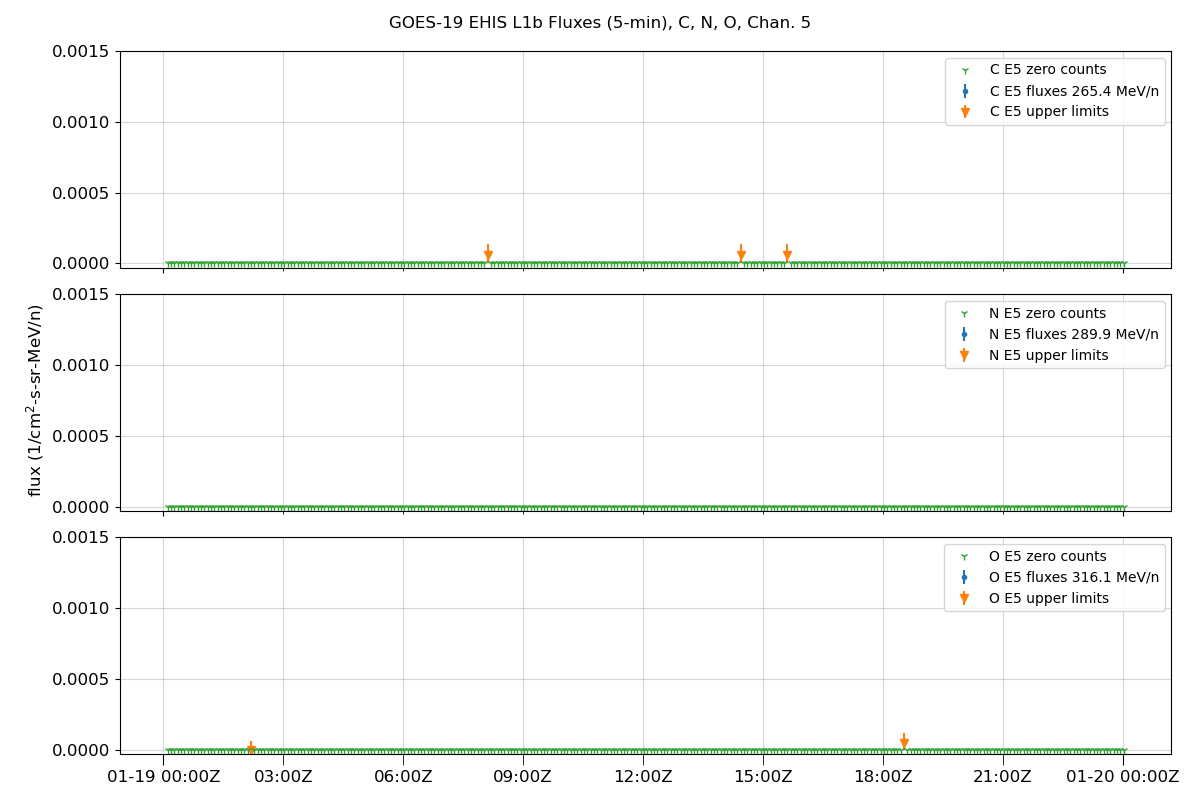
Download and Plot EHIS L1b Data

Download, read, and plot flux of ion species from EHIS L1b data.

Import modules

import matplotlib.pyplot as plt
import matplotlib.dates as mdates
import netCDF4 as nc
import numpy as np
import os
import requests
import cftime

Relevant data files can be downloaded here. Note: To run this code, it may be necessary to update the filename version string (e.g. “v0-0-2”) to match available files.

sat_num = 19
filename = f"ops_seis-l1b-ehis_g{sat_num}_d20260119_v0-0-2.nc"

# Download `filename` if it does not exist locally
if not os.path.exists(filename):
    with open(filename, "wb") as f:
        url_path = f"https://data.ngdc.noaa.gov/platforms/solar-space-observing-satellites/goes/goes{sat_num}/l1b/seis-l1b-ehis/2026/01/"
        r = requests.get(url_path + filename)
        f.write(r.content)

Load data and get data for selected elements

ehis_data = nc.Dataset(filename)

# Heavy ions, Beryllium (Be) to Copper (Cu)
heavy_ions = nc.chartostring(ehis_data['element_label'][:]).tolist()
print(heavy_ions)

['Be', 'B', 'C', 'N', 'O', 'F', 'Ne', 'Na', 'Mg', 'Al', 'Si', 'P', 'S', 'Cl', 'Ar', 'K', 'Ca', 'Sc', 'Ti', 'V', 'Cr', 'Mn', 'Fe', 'Co', 'Ni', 'Cu']

Get flux data for selected ions

# Select ions
# Above He, the most abundant solar heavy ion species are ['C', 'N', 'O', 'Ne', 'Mg', 'Al', 'Si', 'Fe']
selected_ions = ['C', 'N', 'O']

# Get flux data
selected_ions_idx = [heavy_ions.index(item) for item in selected_ions]

ion_fluxes = ehis_data['BeCu5MinuteDifferentialFluxes'][:].filled(np.nan)
selected_ions_fluxes = ion_fluxes[:, :, selected_ions_idx]

selected_ions_energies = ehis_data['BeCu5MinuteDifferentialEnergyBounds'][:, :, selected_ions_idx]

ion_stat_err = ehis_data['BeCu5MinuteDifferentialFluxStatErrorsBounds'][:].filled(np.nan)
selected_ions_stat_err = ion_stat_err[:, :, selected_ions_idx]

selected_ions_inst_err = ehis_data['BeCu5MinuteDifferentialFluxInstErrors'][:, :, selected_ions_idx]

Get timestamps

# Use average of ELF time for timestamps
avg_elf_time = np.nanmean(ehis_data['ELF_StartStopTime'][:], axis=1)

# Convert J2000 time to python datetime
TIME_UNITS = "seconds since 2000-01-01 12:00:00"
time = cftime.num2pydate(avg_elf_time, TIME_UNITS)

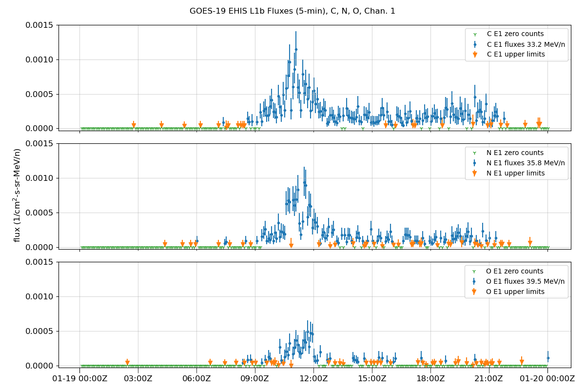
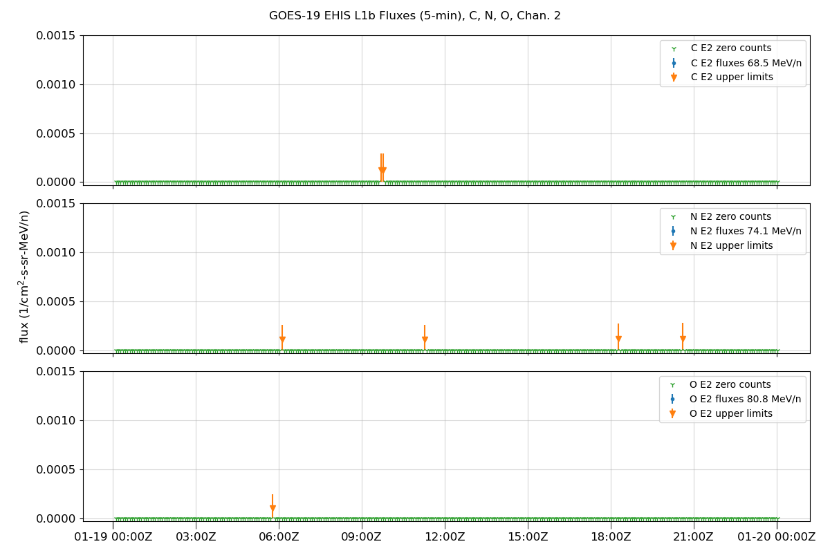
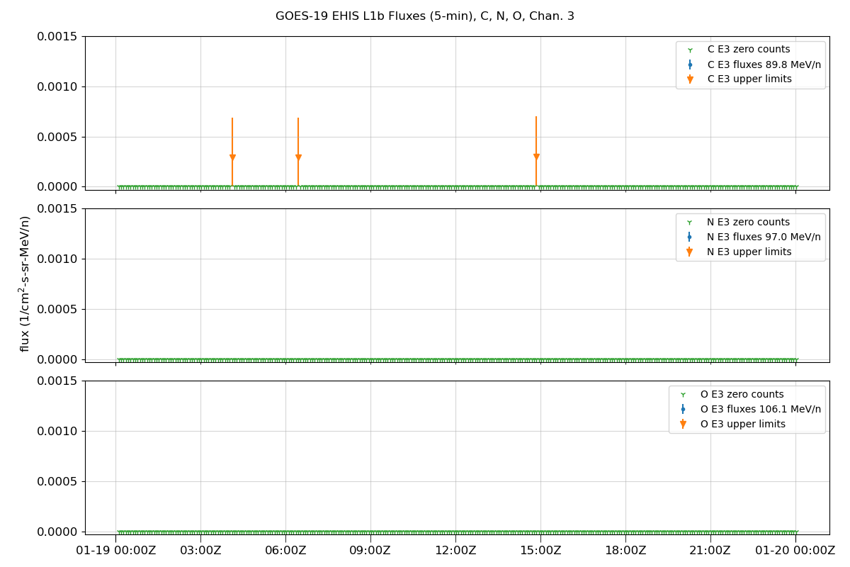
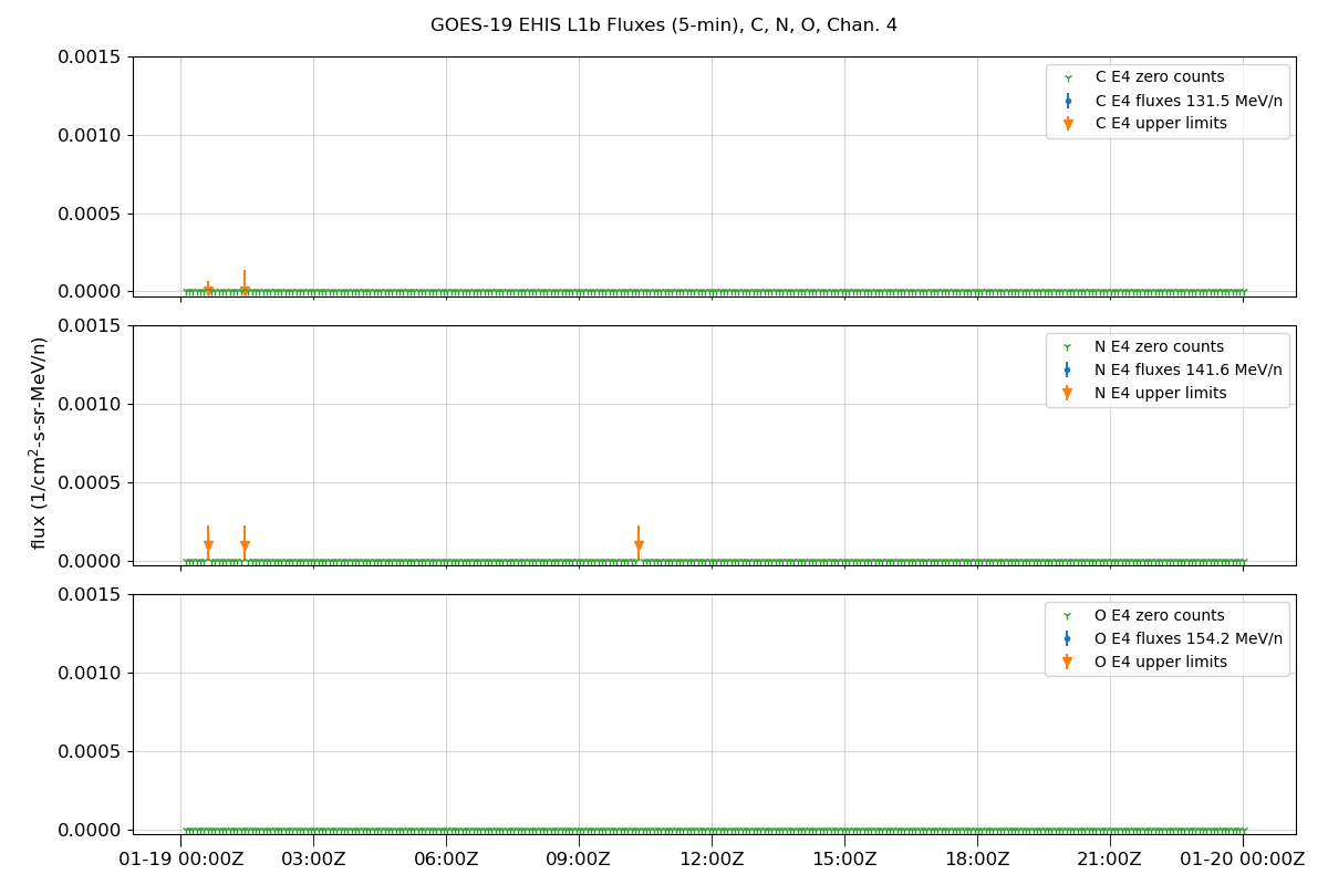
Plot data

NUM_CHANNELS = 5
num_ions = len(selected_ions)

# Use geometric mean of first energies in sequence for plot labels
selected_ions_energies_gm = np.sqrt(selected_ions_energies[0, :, :, 0] * selected_ions_energies[0, :, :, 1])

colors = plt.rcParams['axes.prop_cycle'].by_key()['color']

for chan in range(NUM_CHANNELS):

    fig = plt.figure(chan + 1, figsize=[12, 8])

    for ion_idx in range(num_ions):

        ax = fig.add_subplot(num_ions, 1, ion_idx + 1)

        # Plot where flux > lower stat error
        good_idx = np.where((selected_ions_stat_err[:, chan, ion_idx, 0] < selected_ions_fluxes[:, chan, ion_idx]) &
                            (selected_ions_fluxes[:, chan, ion_idx] > 0.0))

        plt.errorbar(x=time[good_idx],
                     y=np.squeeze(np.atleast_2d(selected_ions_fluxes[good_idx, chan, ion_idx])),
                     yerr=np.atleast_2d(np.squeeze(selected_ions_stat_err[good_idx, chan, ion_idx, :])).T,
                     label=selected_ions[ion_idx] + f' E{chan + 1} fluxes {selected_ions_energies_gm[chan, ion_idx]:.1f} MeV/n',
                     linestyle='none', marker='.', zorder=0, color=colors[0])

        # Plot where flux = lower stat error
        uplims_idx = np.where((selected_ions_stat_err[:, chan, ion_idx, 0] == selected_ions_fluxes[:, chan, ion_idx]) &
                              (selected_ions_fluxes[:, chan, ion_idx] > 0.0))

        plt.errorbar(x=time[uplims_idx],
                     y=np.squeeze(np.atleast_2d(selected_ions_fluxes[uplims_idx, chan, ion_idx])),
                     yerr=np.atleast_2d(np.squeeze(selected_ions_stat_err[uplims_idx, chan, ion_idx, :])).T,
                     label=selected_ions[ion_idx] + ' E{0:1d} upper limits'.format(chan + 1),
                     linestyle='none', marker='v', zorder=0, color=colors[1])

        # Plot where flux = 0
        zeros_idx = np.where(selected_ions_fluxes[:, chan, ion_idx] == 0.0)
        plt.plot(time[zeros_idx], np.squeeze(selected_ions_fluxes[zeros_idx, chan, ion_idx]),
                 label=selected_ions[ion_idx] + ' E{0:1d} zero counts'.format(chan + 1),
                 linestyle='none', marker='1', color=colors[2])

        ax.grid(True, alpha=0.5, which='both')

        # x-axis
        ax.xaxis.set_major_locator(mdates.HourLocator(byhour=0))
        ax.xaxis.set_major_formatter(mdates.DateFormatter('%m-%d %H:%MZ'))
        ax.xaxis.set_minor_locator(mdates.HourLocator(byhour=list(range(3, 24, 3))))
        ax.xaxis.set_minor_formatter(mdates.DateFormatter('%H:%MZ'))
        if ion_idx == num_ions - 1:
            ax.tick_params(axis='x', which='minor', length=8, labelsize=12)
            ax.tick_params(axis='x', which='major', length=8, labelsize=12)
        else:
            ax.tick_params(which='minor', labelbottom=False)
            ax.tick_params(which='major', labelbottom=False)

        # y-axis
        ax.tick_params(axis='y', which='major', labelsize=12)
        plt.ylim([-0.00003, 0.0015])

        plt.legend(loc='upper right', ncol=1, fontsize='10')

        fig.supylabel('flux (1/cm$^2$-s-sr-MeV/n)')
        fig.suptitle(f'GOES-{sat_num} EHIS L1b Fluxes (5-min), {', '.join(selected_ions)}, Chan. {chan + 1}')

    plt.tight_layout()

• 
• 
• 
• 
•